Comparing Clonal Diversity and Overlap

clonalDiversity: Clonal Diversity Quantification

Diversity can be measured for samples or by other variables. clonalDiversity() calculates a specified diversity metric for groups within a dataset. To control for variations in library size, the function can perform bootstrapping with downsampling. It resamples each group to the size of the smallest group and calculates the diversity metric across multiple iterations, returning the mean values.

How `clonalDiversity()` Handles Downsampling and Bootstrapping

It determines the number of clones in the smallest group.
For each group, it performs n.boots iterations (default = 100).
In each iteration, it randomly samples the clones (with replacement) down to the size of the smallest group.
It calculates the selected diversity metric on this downsampled set.
The final reported diversity value is the mean of the results from all bootstrap iterations.
This process can be disabled by setting skip.boots = TRUE.

Available Diversity Metrics (`metric`)

Metric	What it measures	Typical scale	Higher value indicates…
`shannon`	Joint richness + evenness of clonotypes; moderately sensitive to rare clones (entropy of the frequency distribution).	0 → ∞	More distinct clonotypes and a more even clone-size distribution.
`inv.simpson`	Evenness-weighted diversity (inverse Simpson’s D); heavily penalises dominance by a few large clones.	1 → ∞	Few highly dominant clones; diversity spread across many mid-abundance clones.
`norm.entropy`	Shannon entropy divided by ln S (where S = no. clonotypes); removes library-size dependence.	0 → 1	Same interpretation as `shannon`, but comparable across samples of different depths.
`gini.simpson`	1 – Simpson’s D; probability that two reads drawn at random come from different clonotypes.	0 → 1	Greater heterogeneity (higher chance the two reads represent distinct clones).
`chao1`	Estimated richness only (number of clonotypes), correcting for unseen singletons/doubletons.	0 → ∞	More unique clonotypes, regardless of their relative abundances.
`ACE`	Abundance-based Coverage Estimator—alternative richness estimator robust when many clones are rare.	0 → ∞	More unique clonotypes, especially when the repertoire contains many low-frequency clones.
`gini`	Inequality of clone size distribution (Gini Coefficient); measures how unevenly clone sizes are distributed.	0 → 1	Greater inequality; a few highly abundant clones dominate the repertoire.
`d50`	Repertoire dominance; how many of the top clones are needed to constitute 50% of the total library.	1 → ∞	Less dominance by top clones; the repertoire is more evenly distributed.
`hill0`	Richness (Hill number q=0); the total number of unique clonotypes observed in the sample.	0 → ∞	More unique clonotypes (greater raw richness).
`hill1`	Effective number of abundant clonotypes (Hill number q=1); the exponential of Shannon entropy.	1 → ∞	Higher diversity of common clonotypes, balancing richness and evenness.
`hill2`	Effective number of dominant clonotypes (Hill number q=2); equivalent to the inverse Simpson index.	1 → ∞	Higher diversity among the most dominant clonotypes in the repertoire.

Key Parameters for clonalDiversity()

metric: The diversity metric to calculate.
x.axis: An additional metadata variable to group samples along the x-axis.
return.boots: If TRUE, returns all bootstrap values instead of the mean.
skip.boots: If TRUE, disables downsampling and bootstrapping.
n.boots: The number of bootstrap iterations to perform (default is 100).

To calculate Shannon diversity, grouped by sample:

clonalDiversity(combined.TCR, 
                cloneCall = "gene")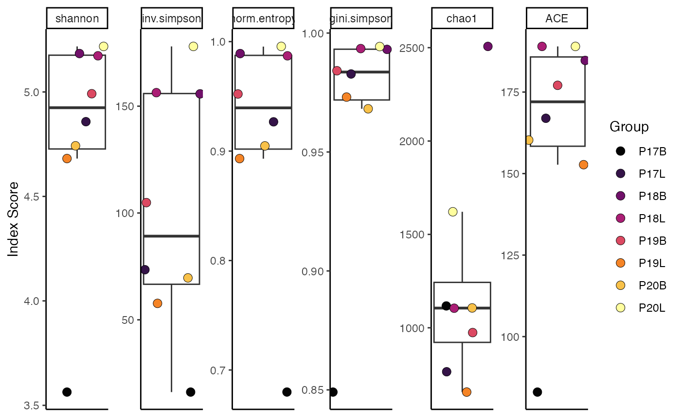

There are two options for grouping in clonalDiversity(): group.by and x.axis.

group.by: Reorganizes the clone information into new groups that the calculation will be based on.
x.axis: Keeps the organization of the clone information the same, but plots along the x-axis for improved visibility or grouping.

First, add a “Patient” variable to combined.TCR

combined.TCR <- addVariable(combined.TCR, 
                            variable.name = "Patient", 
                             variables = c("P17", "P17", "P18", "P18", 
"P19","P19", "P20", "P20"))

Now, calculate Inverse Simpson diversity, grouped by “Patient”:

clonalDiversity(combined.TCR, 
                cloneCall = "gene", 
                group.by = "Patient", 
                metric = "inv.simpson")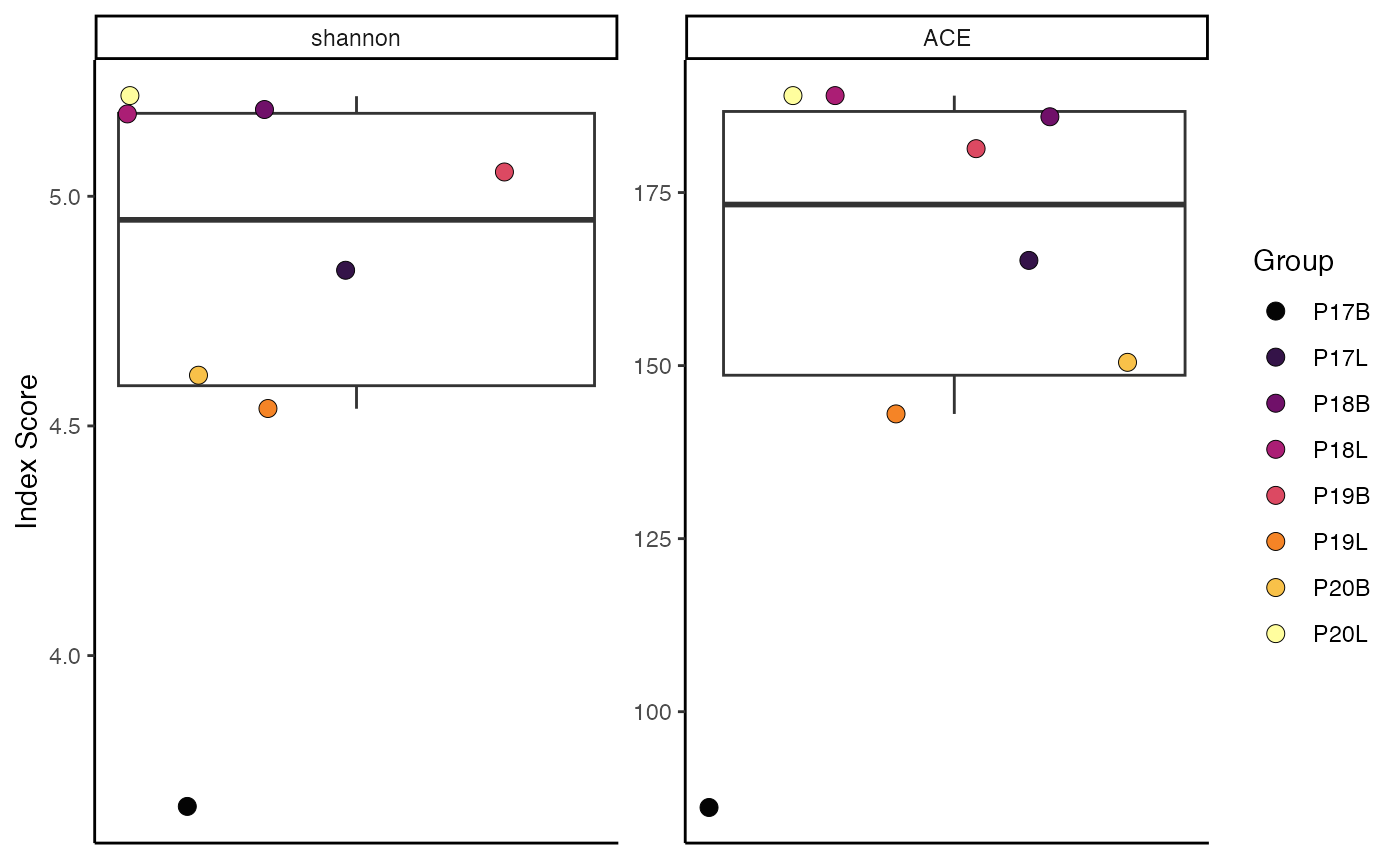

Calculate Inverse Simpson diversity with “Patient” on the x-axis, keeping the original grouping:

clonalDiversity(combined.TCR, 
                cloneCall = "gene", 
                x.axis = "Patient", 
                metric = "inv.simpson")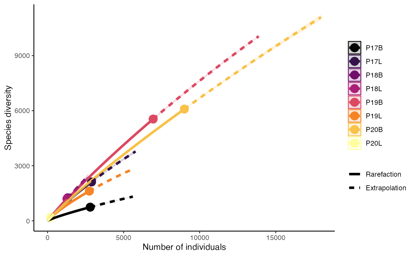

clonalDiversity() functions in quantifying and comparing the diversity of immune repertoires across different samples or experimental conditions. By implementing bootstrapping and offering a wide range of diversity metrics, it provides robust and comparable measures of clonal richness and evenness, which are fundamental for understanding immune responses and disease states

clonalRarefaction: Sampling-based Extrapolation

clonalRarefaction() uses Hill numbers to estimate rarefaction, or estimating species richness, based on the abundance of clones across groupings. The underlying rarefaction calculation uses the observed receptor abundance to compute diversity. This function relies on the iNEXT R package.

Hill Numbers and Their Interpretation

0: Species richness
1: Shannon Diversity
2: Simpson Diversity

plot.type Options

1: Sample-size-based rarefaction/extrapolation curve
2: Sample completeness curve
3: Coverage-based rarefaction/extrapolation curve

Key Parameter(s) for clonalRarefaction()

plot.type: The type of plot to generate.
hill.numbers: The Hill numbers to be plotted (0, 1, or 2).
n.boots: The number of bootstrap replicates used to derive confidence intervals (default is 20).

This function relies on the iNEXT with the accompanying manuscript. Like the other wrapping functions in scRepertoire, please cite the original work. The sample completeness curve (plot.type = 2), may not show full sample coverage due to the size/diversity of the input data.

Rarefaction using Species Richness (q = 0)

clonalRarefaction(combined.TCR,
                  plot.type = 1,
                  hill.numbers = 0,
                  n.boots = 2)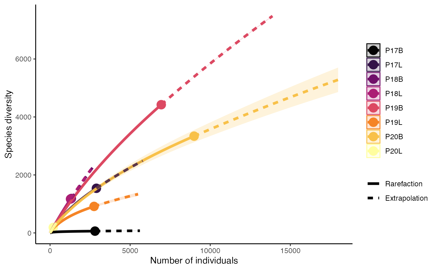

clonalRarefaction(combined.TCR,
                  plot.type = 2,
                  hill.numbers = 0,
                  n.boots = 2)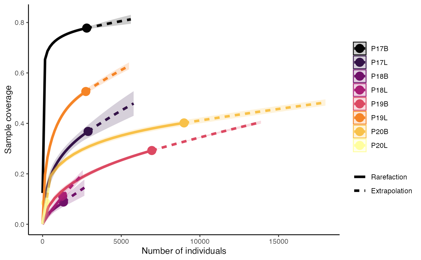

clonalRarefaction(combined.TCR,
                  plot.type = 3,
                  hill.numbers = 0,
                  n.boots = 2)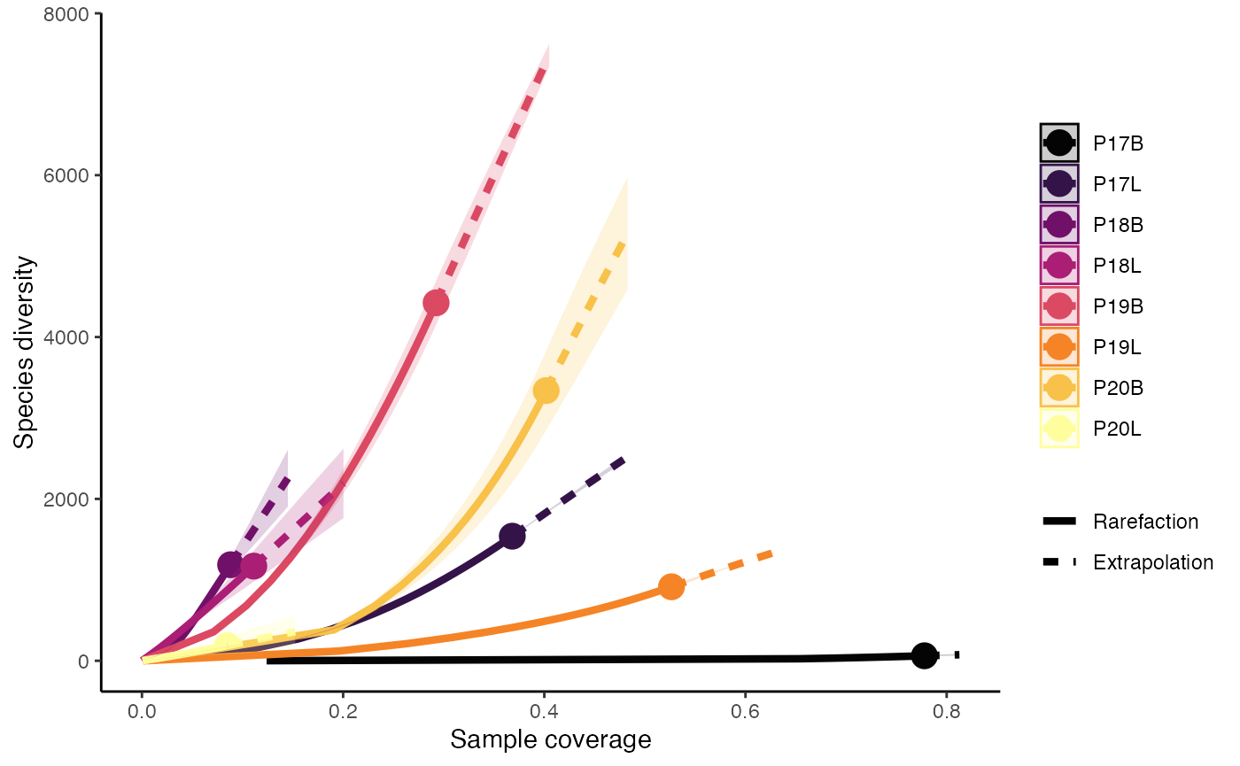

Rarefaction using Shannon Diversity (q = 1)

clonalRarefaction(combined.TCR,
                  plot.type = 1,
                  hill.numbers = 1,
                  n.boots = 2)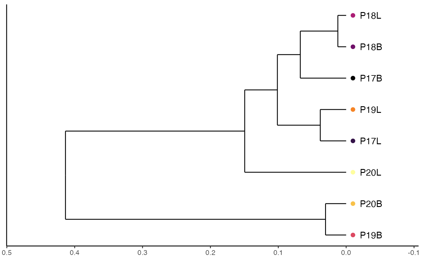

clonalRarefaction(combined.TCR,
                  plot.type = 2,
                  hill.numbers = 1,
                  n.boots = 2)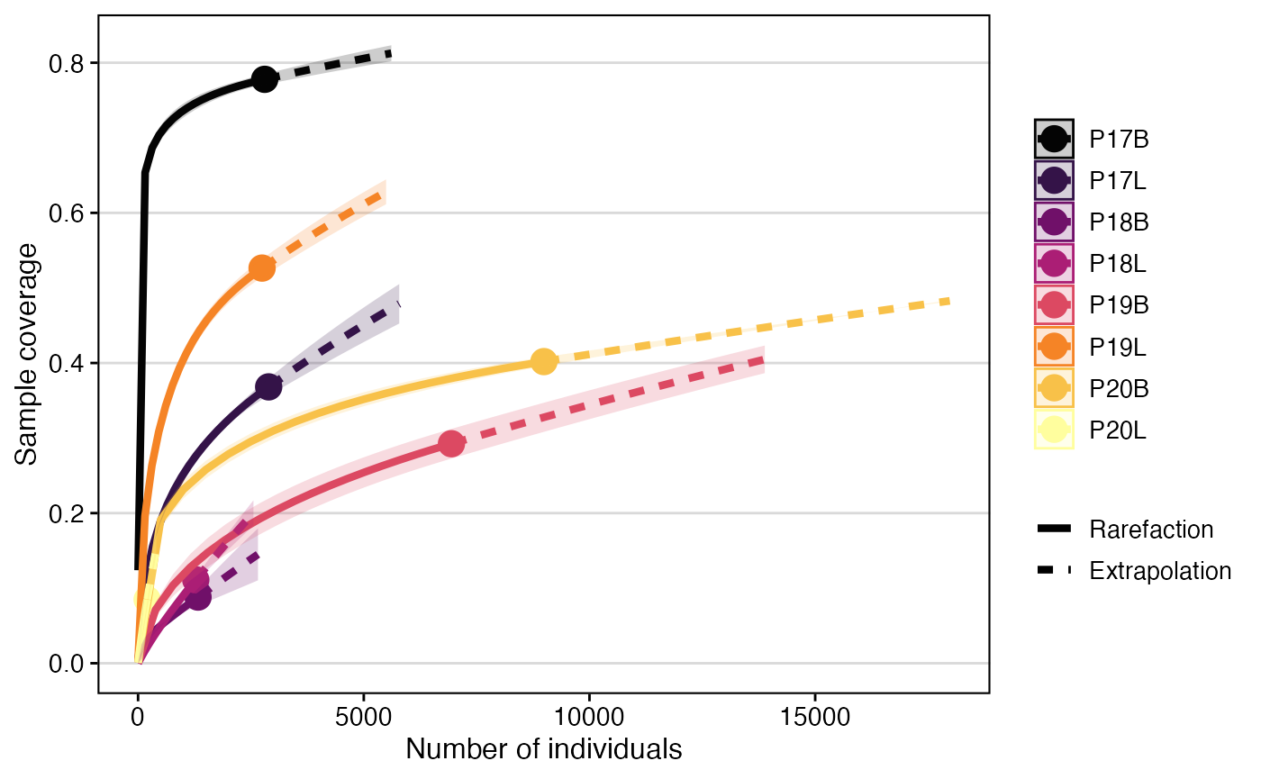

clonalRarefaction(combined.TCR,
                  plot.type = 3,
                  hill.numbers = 1,
                  n.boots = 2)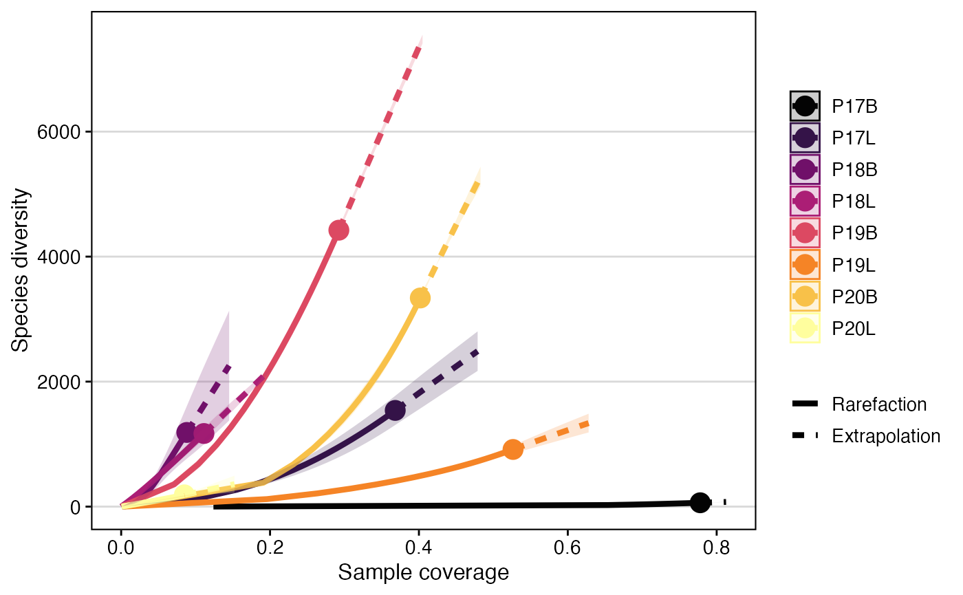

clonalRarefaction() provides robust estimates of immune repertoire diversity, allowing for comparison of richness and effective diversity across samples, even with varying sequencing depths. By visualizing rarefaction and extrapolation curves, researchers can assess the completeness of their sampling and make fair comparisons of diversity, which is essential for understanding immune complexity.

clonalSizeDistribution: Advanced Modeling Of Clonal Composition

Another method for modeling the repertoire distribution is a discrete gamma-GPD spliced threshold model, proposed by Koch et al. The spliced model models the repertoire and allows for the application of a power law distribution for larger clonal-expanded sequences and a Poisson distribution for smaller clones. After fitting the models, repertoires can be compared using Euclidean distance. If using this function, please read/cite Koch et al. and check out the powerTCR R package.

Key Parameter(s) for clonalSizeDistribution()

method: The agglomeration method for hierarchical clustering (e.g., “ward.D2”).

To model the clonal size distribution using amino acid clone calls and hierarchical clustering with the “ward.D2” method:

clonalSizeDistribution(combined.TCR, 
                       cloneCall = "aa", 
                       method= "ward.D2")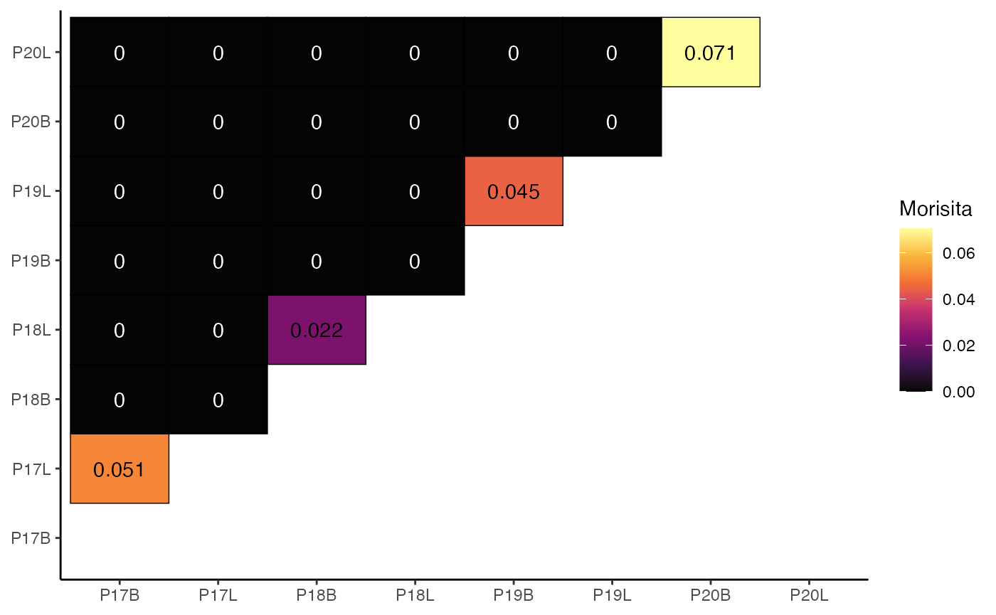

clonalSizeDistribution() offers a sophisticated approach to modeling immune repertoire composition, distinguishing between the distribution of rare and expanded clones. By applying a spliced statistical model, it provides a more accurate representation of the repertoire’s underlying clonal architecture, enabling robust comparisons and a deeper understanding of immune system dynamics.

clonalOverlap: Exploring Sequence Overlap

If you are interested in measures of similarity between the samples loaded into scRepertoire, using clonalOverlap() can assist in the visualization. The underlying clonalOverlap() calculation varies by the method parameter.

`method` Parameters for `clonalOverlap()`

overlap - Overlap coefficient
morisita - Morisita’s overlap index
jaccard - Jaccard index
cosine - Cosine similarity
raw - Exact number of overlapping clones

To calculate and visualize the Morisita overlap index using strict clone calls:

clonalOverlap(combined.TCR, 
              cloneCall = "strict", 
              method = "morisita")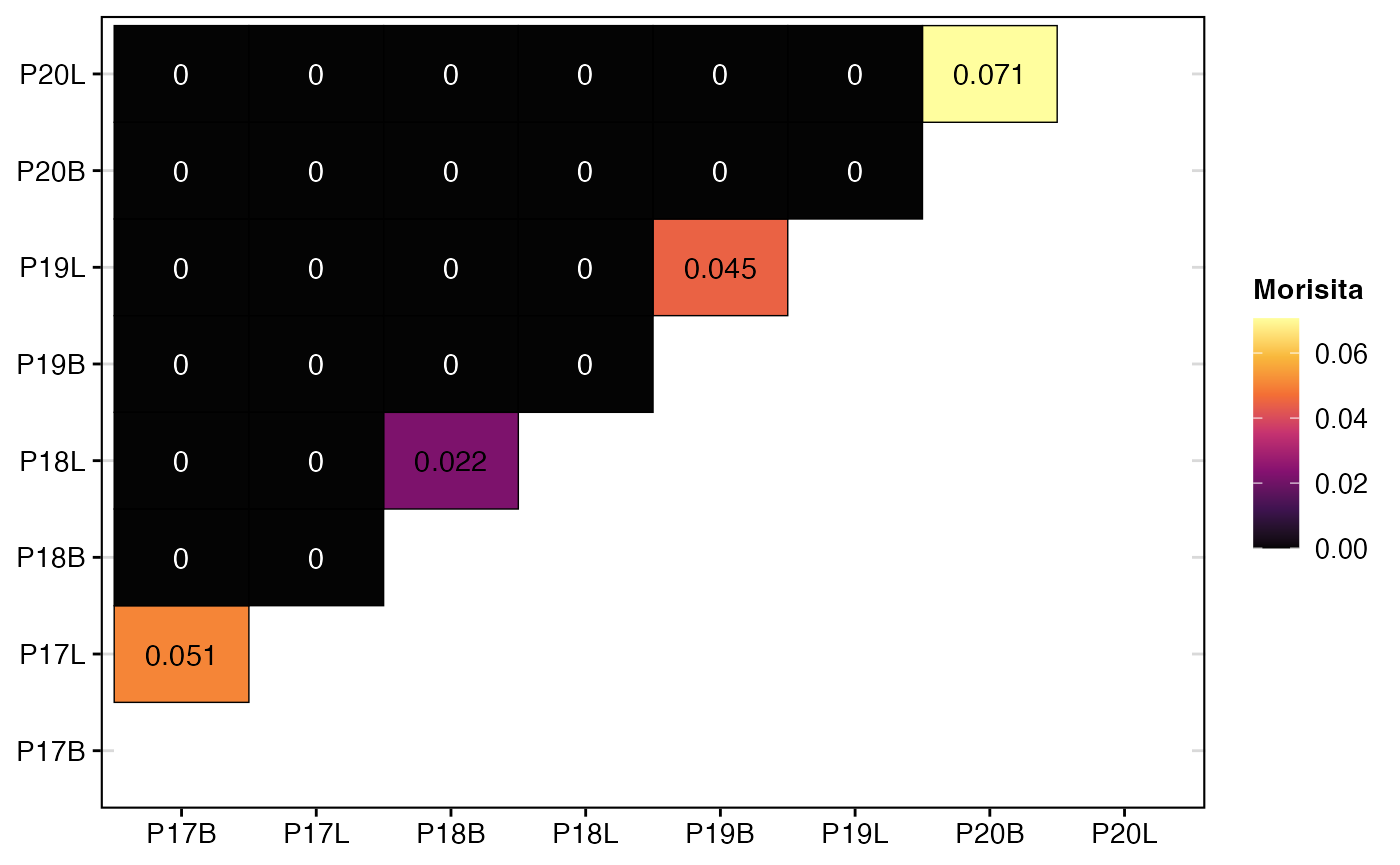

To calculate and visualize the raw number of overlapping clones using strict clone calls:

clonalOverlap(combined.TCR, 
              cloneCall = "strict", 
              method = "raw")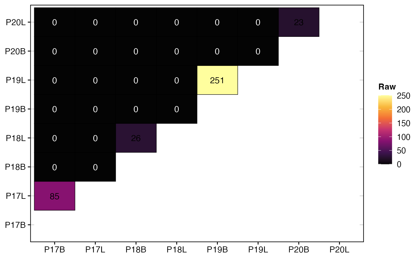

clonalOverlap() is a tool for assessing the similarity and shared clonotypes between different immune repertoires. By offering various quantitative methods and a clear heatmap visualization, it allows researchers to identify the degree of overlap, providing insights into shared immune responses, cross-reactivity, or the impact of different treatments on clonal composition.

Compiled: July 31, 2025