Examining the clonal overlap between groups or samples

This functions allows for the calculation and visualizations of various overlap metrics for clones. The methods include overlap coefficient (overlap), Morisita's overlap index (morisita), Jaccard index (jaccard), cosine similarity (cosine) or the exact number of clonal overlap (raw).

Usage

clonalOverlap(
  input.data,
  clone.call = NULL,
  method = c("overlap", "morisita", "jaccard", "cosine", "raw"),
  chain = "both",
  group.by = NULL,
  order.by = NULL,
  export.table = NULL,
  palette = "inferno",
  cloneCall = NULL,
  exportTable = NULL,
  ...
)

Arguments

input.data: The product of combineTCR(), combineBCR(), or combineExpression()
clone.call: Defines the clonal sequence grouping. Accepted values are: gene (VDJC genes), nt (CDR3 nucleotide sequence), aa (CDR3 amino acid sequence), or strict (VDJC + nt). A custom column header can also be used.
method: The method to calculate the overlap, morisita, jaccard, cosine indices or raw for the base numbers
chain: The TCR/BCR chain to use. Use both to include both chains (e.g., TRA/TRB). Accepted values: TRA, TRB, TRG, TRD, IGH, IGL, IGK, Light (for both light chains), or both (for TRA/B and Heavy/Light).
group.by: A column header in the metadata or lists to group the analysis by (e.g., "sample", "treatment"). If NULL, data will be analyzed by list element or active identity in the case of single-cell objects.
order.by: A character vector defining the desired order of elements of the group.by variable. Alternatively, use alphanumeric to sort groups automatically.
export.table: If TRUE, returns a data frame or matrix of the results instead of a plot.
palette: Colors to use in visualization - input any hcl.pals
cloneCall: Use clone.call instead.
exportTable: Use export.table instead.
...: Additional arguments passed to the ggplot theme

Value

A ggplot object visualizing clonal overlap or a data.frame if exportTable = TRUE.

Details

The formulas for the indices are as follows:

Overlap Coefficient: $$overlap = \frac{\sum \min(a, b)}{\min(\sum a, \sum b)}$$

Raw Count Overlap: $$raw = \sum \min(a, b)$$

Morisita Index: $$morisita = \frac{\sum a b}{(\sum a)(\sum b)}$$

Jaccard Index: $$jaccard = \frac{\sum \min(a, b)}{\sum a + \sum b - \sum \min(a, b)}$$

Cosine Similarity: $$cosine = \frac{\sum a b}{\sqrt{(\sum a^2)(\sum b^2)}}$$

Where:

$a$ and $b$ are the abundances of species $i$ in groups A and B, respectively.

Examples

# Making combined contig data
combined <- combineTCR(contig_list, 
                        samples = c("P17B", "P17L", "P18B", "P18L", 
                                    "P19B","P19L", "P20B", "P20L"))

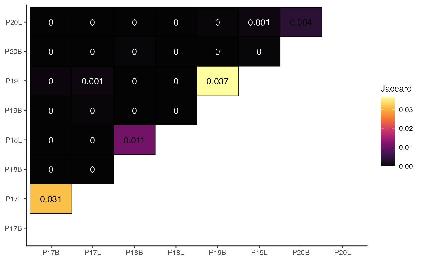
# Using clonalOverlap()
clonalOverlap(combined,
              clone.call = "aa",
              method = "jaccard")