Visualizing Clonal Dynamics

clonalHomeostasis: Examining Clonal Space

By examining the clonal space, we effectively look at the relative space occupied by clones at specific proportions. Another way to think about this would be to consider the total immune receptor sequencing run as a measuring cup. In this cup, we will fill liquids of different viscosity—or different numbers of clonal proportions. Clonal space homeostasis asks what percentage of the cup is filled by clones in distinct proportions (or liquids of different viscosity, to extend the analogy). The proportional cut points are set under the cloneSize variable in the function and can be adjusted.

Default cloneSize Bins

• Rare: 0 to 0.0001
• Small: 0.0001 to 0.001
• Medium: 0.001 to 0.01
• Large: 0.01 to 0.1
• Hyperexpanded: 0.1 to 1

To visualize clonal homeostasis using gene clone calls with default cloneSize bins:

clonalHomeostasis(combined.TCR, 
                  cloneCall = "gene")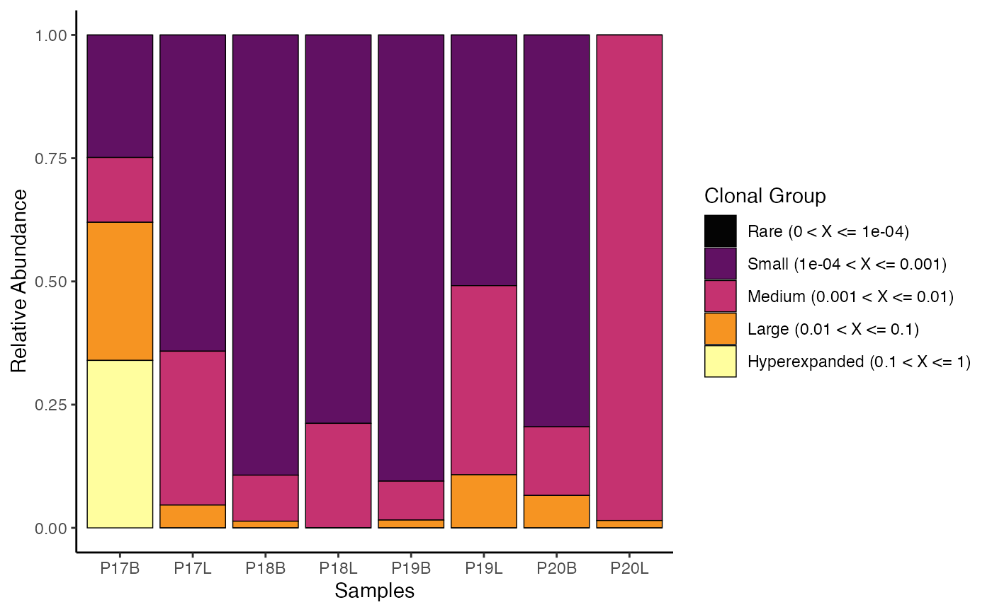

We can reassign the proportional cut points for cloneSize, which can drastically alter the visualization and analysis

clonalHomeostasis(combined.TCR, 
                  cloneCall = "gene",
                  cloneSize = c(Rare = 0.001, Small = 0.01, Medium = 0.1, 
                                Large = 0.3, Hyperexpanded = 1))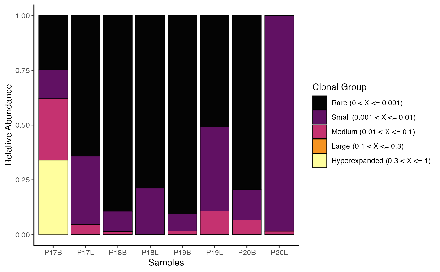

In addition, we can use the group.by parameter to look at the relative proportion of clones between groups, such as by tissue type. First, ensure the “Type” variable is added to combined.TCR:

combined.TCR <- addVariable(combined.TCR, 
                            variable.name = "Type", 
                            variables = rep(c("B", "L"), 4))

Now, visualize clonal homeostasis grouped by “Type”:

clonalHomeostasis(combined.TCR, 
                  group.by = "Type",
                  cloneCall = "gene")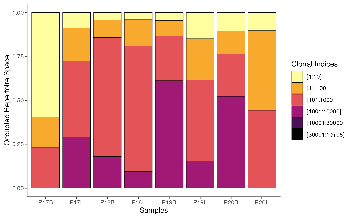

clonalHomeostasis() provides an assessment of how different “sizes” of clones (based on their proportional abundance) contribute to the overall repertoire. This visualization helps to identify shifts in repertoire structure, such as expansion of large clones in response to infection or contraction in chronic conditions, offering insights into immune system activity and health.

clonalProportion: Examining Space Occupied by Ranks of Clones

Like clonal space homeostasis, clonalProportion() also categorizes clones into separate bins. The key difference is that instead of looking at the relative proportion of the clone to the total, clonalProportion() ranks the clones by their total count or frequency of occurrence and then places them into predefined bins.

The clonalSplit parameter represents the ranking of clonotypes. For example, 1:10 refers to the top 10 clonotypes in each sample. The default bins are set under the clonalSplit variable and can be adjusted.

Default clonalSplit Bins

• 10 (top 1-10 clones)
• 100: (top 11-100 clones)
• 1000: (top 101-1000 clones)
• 10000: (top 1001-10000 clones)
• 30000: (top 10001-30000 clones)
• 100000: (top 30001-100000 clones)

To visualize the clonal proportion using gene clone calls with default clonalSplit bins:

clonalProportion(combined.TCR, 
                 cloneCall = "gene")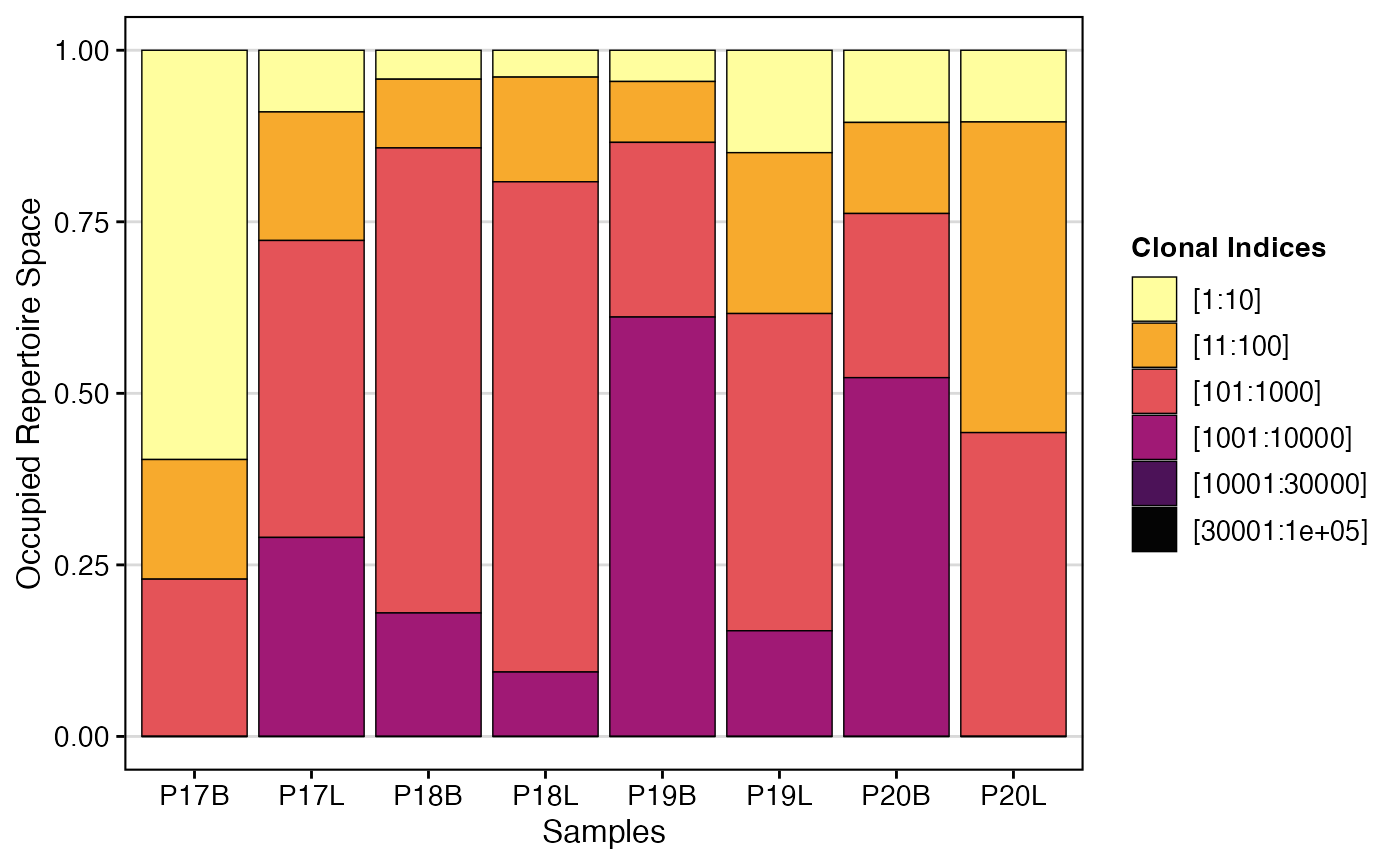 

To visualize clonal proportion using nt (nucleotide) clone calls with custom clonalSplit bins:

clonalProportion(combined.TCR, 
                 cloneCall = "nt",
                 clonalSplit = c(1, 5, 10, 100, 1000, 10000))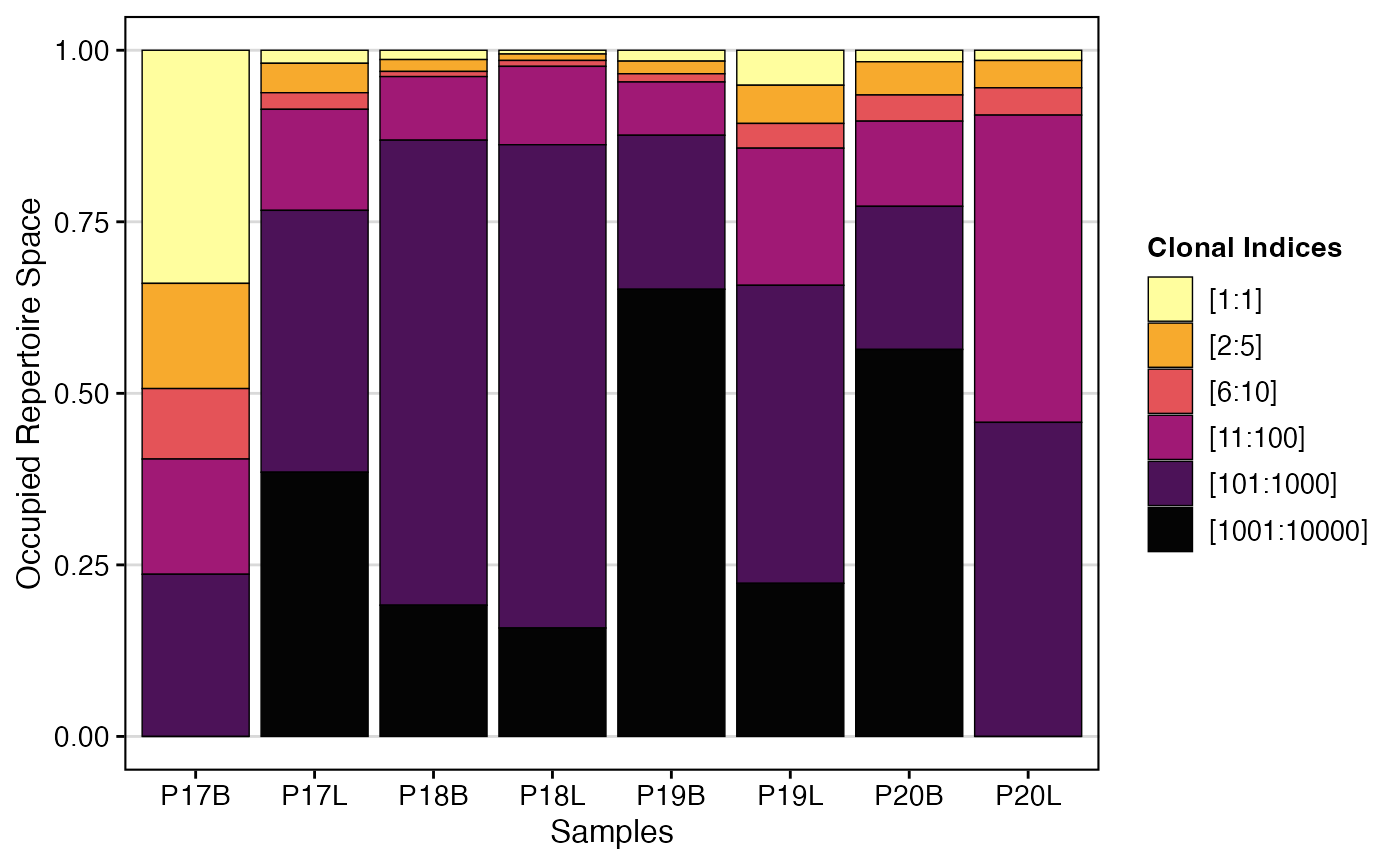 

clonalProportion() complements clonalHomeostasis() by providing a perspective on how the “richest” (most abundant) clones contribute to the overall repertoire space. By segmenting clones into rank-based bins, it helps identify whether a few highly expanded clones or a larger number of moderately expanded clones dominate the immune response, offering distinct insights into repertoire structure and dynamics.