Calculate Clonal Diversity

Arguments

input.data

The product of combineTCR(), combineBCR(), or combineExpression().

cloneCall

Defines the clonal sequence grouping. Accepted values are: gene (VDJC genes), nt (CDR3 nucleotide sequence), aa (CDR3 amino acid sequence), or strict (VDJC + nt). A custom column header can also be used.

metric

The diversity metric to calculate. Must be a single string from the list of available metrics (see Details).

chain

The TCR/BCR chain to use. Use both to include both chains (e.g., TRA/TRB). Accepted values: TRA, TRB, TRG, TRD, IGH, IGL (for both light chains), both.

group.by

A column header in the metadata or lists to group the analysis by (e.g., "sample", "treatment"). If NULL, data will be analyzed by list element or active identity in the case of single-cell objects.

order.by

A character vector defining the desired order of elements of the group.by variable. Alternatively, use alphanumeric to sort groups automatically.

x.axis

An additional metadata variable to group samples along the x-axis.

exportTable

If TRUE, returns a data frame or matrix of the results instead of a plot.

palette

Colors to use in visualization - input any hcl.pals.

n.boots

The number of bootstrap iterations to perform (default is 100).

return.boots

If TRUE, returns all bootstrap values instead of the mean. Automatically enables exportTable.

skip.boots

If TRUE, disables downsampling and bootstrapping. The metric will be calculated on the full dataset for each group. Defaults to FALSE.

...

Additional arguments passed to the ggplot theme

Value

A ggplot object visualizing the diversity metric, or a data.frame if exportTable = TRUE.

Details

The function operates by first splitting the dataset by the specified group.by variable.

Downsampling and Bootstrapping: To make a fair comparison between groups of different sizes, diversity metrics often require normalization. This function implements this by downsampling.

1. It determines the number of clones in the smallest group.

2. For each group, it performs n.boots iterations (default = 100).

3. In each iteration, it randomly samples the clones (with replacement) down to the size of the smallest group.

4. It calculates the selected diversity metric on this downsampled set.

5. The final reported diversity value is the mean of the results from all bootstrap iterations.

This process can be disabled by setting skip.boots = TRUE.

Available Diversity Metrics (metric): The function uses a registry of metrics imported from the immApex package. You can select one of the following:

• "shannon": Shannon's Entropy. See shannon_entropy.

• "inv.simpson": Inverse Simpson Index. See inv_simpson.

• "gini.simpson": Gini-Simpson Index. See gini_simpson.

• "norm.entropy": Normalized Shannon Entropy. See norm_entropy.

• "pielou": Pielou's Evenness (same as norm.entropy). See pielou_evenness.

• "ace": Abundance-based Coverage Estimator. See ace_richness.

• "chao1": Chao1 Richness Estimator. See chao1_richness.

• "gini": Gini Coefficient for inequality. See gini_coef.

• "d50": The number of top clones making up 50% of the library. See d50_dom.

• "hill0", "hill1", "hill2": Hill numbers of order 0, 1, and 2. See hill_q.

Author

Andrew Malone, Nick Borcherding, Nathan Vanderkraan

Examples

# Making combined contig data
combined <- combineTCR(contig_list,
                       samples = c("P17B", "P17L", "P18B", "P18L",
                                   "P19B","P19L", "P20B", "P20L"))

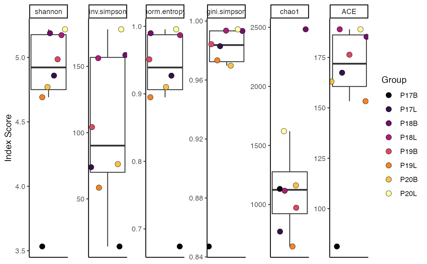
# Calculate Shannon diversity, grouped by sample
clonalDiversity(combined, 
                cloneCall = "gene", 
                metric = "shannon")


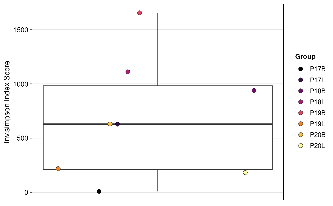
# Calculate Inverse Simpson without bootstrapping
clonalDiversity(combined, 
                cloneCall = "aa", 
                metric = "inv.simpson", 
                skip.boots = TRUE)