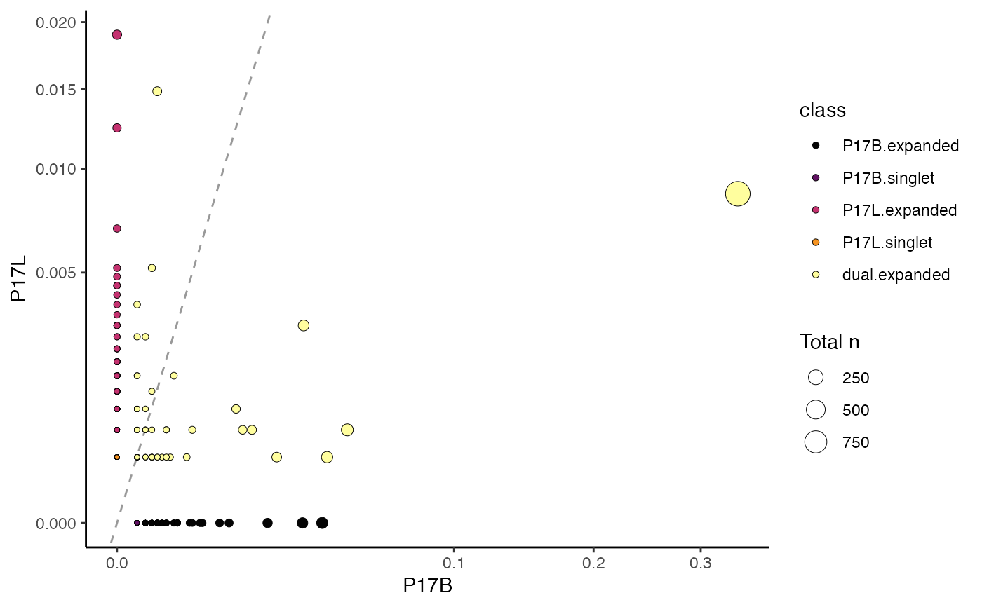
This function produces a scatter plot directly comparing the specific clones between two samples. The clones will be categorized by counts into singlets or expanded, either exclusive or shared between the selected samples.
Usage
clonalScatter(
  input.data,
  clone.call = NULL,
  x.axis = NULL,
  y.axis = NULL,
  chain = "both",
  dot.size = "total",
  group.by = NULL,
  graph = "proportion",
  export.table = NULL,
  palette = "inferno",
  cloneCall = NULL,
  exportTable = NULL,
  ...
)
Arguments
- input.data
The product of
combineTCR(),combineBCR(), orcombineExpression().- clone.call
Defines the clonal sequence grouping. Accepted values are:
gene(VDJC genes),nt(CDR3 nucleotide sequence),aa(CDR3 amino acid sequence), orstrict(VDJC + nt). A custom column header can also be used.- x.axis
name of the list element to appear on the x.axis.
- y.axis
name of the list element to appear on the y.axis.
- chain
The TCR/BCR chain to use. Use
bothto include both chains (e.g., TRA/TRB). Accepted values:TRA,TRB,TRG,TRD,IGH,IGL,IGK,Light(for both light chains), orboth(for TRA/B and Heavy/Light).- dot.size
either total or the name of the list element to use for size of dots.
- group.by
A column header in the metadata or lists to group the analysis by (e.g., "sample", "treatment"). If
NULL, data will be analyzed by list element or active identity in the case of single-cell objects.- graph
graph either the clonal "proportion" or "count".
- export.table
If
TRUE, returns a data frame or matrix of the results instead of a plot.- palette
Colors to use in visualization - input any hcl.pals.
- cloneCall
![[Deprecated]](figures/lifecycle-deprecated.svg) Use
Use clone.callinstead.- exportTable
- Use
export.tableinstead. - ...
Additional arguments passed to the ggplot theme
Value
A ggplot object visualizing clonal dynamics between two groupings or
a data.frame if exportTable = TRUE.
Examples
#Making combined contig data
combined <- combineTCR(contig_list,
                        samples = c("P17B", "P17L", "P18B", "P18L",
                                    "P19B","P19L", "P20B", "P20L"))

# Using clonalScatter()
clonalScatter(combined,
              x.axis = "P17B",
              y.axis = "P17L",
              graph = "proportion")