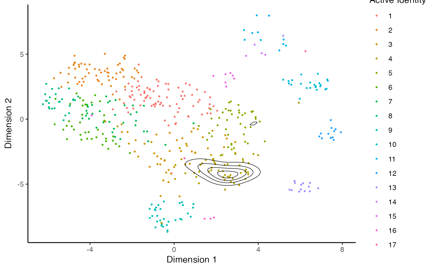
This function allows the user to visualize the clonal expansion by overlaying the cells with specific clonal frequency onto the dimensional reduction plots in Seurat. Credit to the idea goes to Drs Andreatta and Carmona and their work with ProjectTIL.
Usage
clonalOverlay(
  sc.data,
  reduction = NULL,
  cut.category = "clonalFrequency",
  cutpoint = 30,
  bins = 25,
  pt.size = 0.5,
  pt.alpha = 1,
  facet.by = NULL,
  ...
)
Arguments
- sc.data
The single-cell object after
combineExpression().- reduction
The dimensional reduction to visualize.
- cut.category
Meta data variable of the single-cell object to use for filtering.
- cutpoint
The overlay cut point to include, this corresponds to the cut.category variable in the meta data of the single-cell object.
- bins
The number of contours to the overlay
- pt.size
The point size for plotting (default is 0.5)
- pt.alpha
The alpha value for plotting (default is 1)
- facet.by
meta data variable to facet the comparison
- ...
Additional arguments passed to the ggplot theme
Value
A ggplot object visualizing distributions of clones along a dimensional reduction within the single-cell object
Examples
# Getting the combined contigs
combined <- combineTCR(contig_list,
                        samples = c("P17B", "P17L", "P18B", "P18L",
                                    "P19B","P19L", "P20B", "P20L"))
# Getting a sample of a Seurat object
scRep_example <- get(data("scRep_example"))

# Using combineExpresion()
scRep_example <- combineExpression(combined,
                                   scRep_example)

# Using clonalOverlay()
clonalOverlay(scRep_example,
              reduction = "umap",
              cutpoint = 3,
              bins = 5)