Plot cloneSize by Variable in Single-Cell Objects

View the count of clones frequency group in Seurat or SCE object meta data after combineExpression(). The visualization will take the new meta data variable cloneSize and plot the number of cells with each designation using a secondary variable, like cluster. Credit to the idea goes to Drs. Carmona and Andreatta and their work with ProjectTIL.

clonalOccupy(
  sc.data,
  x.axis = "ident",
  label = TRUE,
  facet.by = NULL,
  order.by = NULL,
  proportion = FALSE,
  na.include = FALSE,
  exportTable = FALSE,
  palette = "inferno",
  ...
)

Arguments

sc.data: The single-cell object after combineExpression()
x.axis: The variable in the meta data to graph along the x.axis.
label: Include the number of clone in each category by x.axis variable
facet.by: The column header used for faceting the graph
order.by: A character vector defining the desired order of elements of the group.by variable. Alternatively, use alphanumeric to sort groups automatically.
proportion: Convert the stacked bars into relative proportion
na.include: Visualize NA values or not
exportTable: If TRUE, returns a data frame or matrix of the results instead of a plot.
palette: Colors to use in visualization - input any hcl.pals
...: Additional arguments passed to the ggplot theme

Value

Stacked bar plot of counts of cells by clone frequency group

Examples

# Getting the combined contigs
combined <- combineTCR(contig_list, 
                        samples = c("P17B", "P17L", "P18B", "P18L", 
                                    "P19B","P19L", "P20B", "P20L"))

# Getting a sample of a Seurat object
scRep_example <- get(data("scRep_example"))

# Using combineExpresion()
scRep_example <- combineExpression(combined, scRep_example)

# Using clonalOccupy
clonalOccupy(scRep_example, x.axis = "ident")

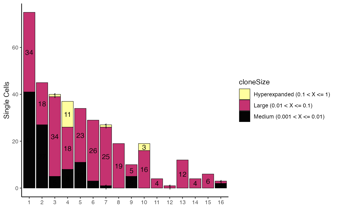table <- clonalOccupy(scRep_example, x.axis = "ident", exportTable = TRUE)