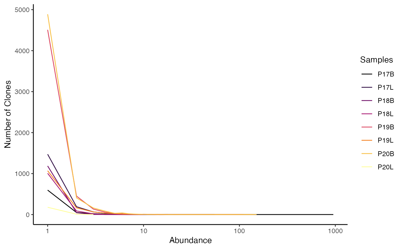
Displays the number of clones at specific frequencies by sample
or group. Visualization can either be a line graph (
scale = FALSE) using calculated numbers or density
plot (scale = TRUE). Multiple sequencing runs can
be group together using the group parameter. If a matrix
output for the data is preferred, set
export.table = TRUE.
Usage
clonalAbundance(
  input.data,
  clone.call = NULL,
  chain = "both",
  scale = FALSE,
  group.by = NULL,
  order.by = NULL,
  export.table = NULL,
  palette = "inferno",
  cloneCall = NULL,
  exportTable = NULL,
  ...
)
Arguments
- input.data
The product of
combineTCR(),combineBCR(), orcombineExpression().- clone.call
Defines the clonal sequence grouping. Accepted values are:
gene(VDJC genes),nt(CDR3 nucleotide sequence),aa(CDR3 amino acid sequence), orstrict(VDJC + nt). A custom column header can also be used.- chain
The TCR/BCR chain to use. Use
bothto include both chains (e.g., TRA/TRB). Accepted values:TRA,TRB,TRG,TRD,IGH,IGL,IGK,Light(for both light chains), orboth(for TRA/B and Heavy/Light).- scale
Converts the graphs into density plots in order to show relative distributions.
- group.by
A column header in the metadata or lists to group the analysis by (e.g., "sample", "treatment"). If
NULL, data will be analyzed by list element or active identity in the case of single-cell objects.- order.by
A character vector defining the desired order of elements of the
group.byvariable. Alternatively, usealphanumericto sort groups automatically.- export.table
If
TRUE, returns a data frame or matrix of the results instead of a plot.- palette
Colors to use in visualization - input any hcl.pals.
- cloneCall
![[Deprecated]](figures/lifecycle-deprecated.svg) Use
Use clone.callinstead.- exportTable
- Use
export.tableinstead. - ...
Additional arguments passed to the ggplot theme
Value
A ggplot object visualizing clonal abundance by group, or a
data.frame if export.table = TRUE.
Examples
# Making combined contig data
combined <- combineTCR(contig_list,
                        samples = c("P17B", "P17L", "P18B", "P18L",
                                    "P19B","P19L", "P20B", "P20L"))

# Using clonalAbundance()
clonalAbundance(combined,
                clone.call = "gene",
                scale = FALSE)