Alluvial Plotting for Single-Cell Object

View the proportional contribution of clones by Seurat or SCE object meta data after combineExpression(). The visualization is based on the ggalluvial package, which requires the aesthetics to be part of the axes that are visualized. Therefore, alpha, facet, and color should be part of the the axes you wish to view or will add an additional stratum/column to the end of the graph.

Usage

alluvialClones(
  sc.data,
  clone.call = NULL,
  chain = "both",
  y.axes = NULL,
  color = NULL,
  facet = NULL,
  alpha = NULL,
  top.clones = NULL,
  min.freq = 0,
  highlight.clones = NULL,
  highlight.color = "red",
  stratum.width = 0.2,
  flow.alpha = 0.5,
  show.labels = TRUE,
  label.size = 2,
  order.strata = NULL,
  export.table = NULL,
  palette = "inferno",
  cloneCall = NULL,
  exportTable = NULL,
  ...
)

Arguments

sc.data

The product of combineExpression().

clone.call

Defines the clonal sequence grouping. Accepted values are: gene (VDJC genes), nt (CDR3 nucleotide sequence), aa (CDR3 amino acid sequence), or strict (VDJC + nt). A custom column header can also be used.

chain

The TCR/BCR chain to use. Use both to include both chains (e.g., TRA/TRB). Accepted values: TRA, TRB, TRG, TRD, IGH, IGL, IGK, Light (for both light chains), or both (for TRA/B and Heavy/Light).

y.axes

The columns that will separate the proportional visualizations.

color

The column header or clone(s) to be highlighted.

facet

The column label to separate.

alpha

The column header to have gradated opacity.

top.clones

Show only the top N clones by frequency. If NULL (default), show all clones.

min.freq

Minimum frequency threshold for displaying flows. Clones appearing fewer than this many times are filtered out.

highlight.clones

Character vector of specific clone sequences to highlight. These clones will be colored distinctly while others are shown in gray.

highlight.color

Color to use for highlighted clones (default: "red").

stratum.width

Width of the stratum bars (default: 0.2).

flow.alpha

Transparency of the flows (default: 0.5). Highlighted clones use full opacity.

show.labels

If TRUE (default), display stratum labels.

label.size

Text size for stratum labels (default: 2).

order.strata

Named list specifying the order of levels within each stratum. Names should match column names in y.axes.

export.table

If TRUE, returns a data frame of the results instead of a plot.

palette

Colors to use in visualization - input any hcl.pals.

cloneCall

Use clone.call instead.

exportTable

Use export.table instead.

...

Additional arguments passed to the ggplot theme

Value

A ggplot object visualizing categorical distribution of clones, or a data.frame if export.table = TRUE.

Examples

# Getting the combined contigs
combined <- combineTCR(contig_list,
                        samples = c("P17B", "P17L", "P18B", "P18L",
                                    "P19B","P19L", "P20B", "P20L"))

# Getting a sample of a Seurat object
scRep_example <- get(data("scRep_example"))

# Using combineExpresion()
scRep_example <- combineExpression(combined, scRep_example)
scRep_example$Patient <- substring(scRep_example$orig.ident, 1,3)

# Using alluvialClones()
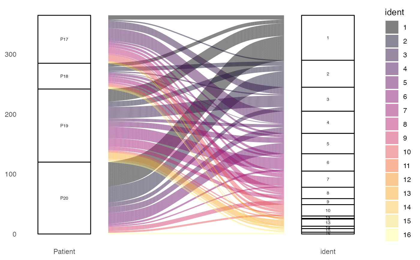
alluvialClones(scRep_example,
                   clone.call = "gene",
                   y.axes = c("Patient", "ident"),
                   color = "ident")


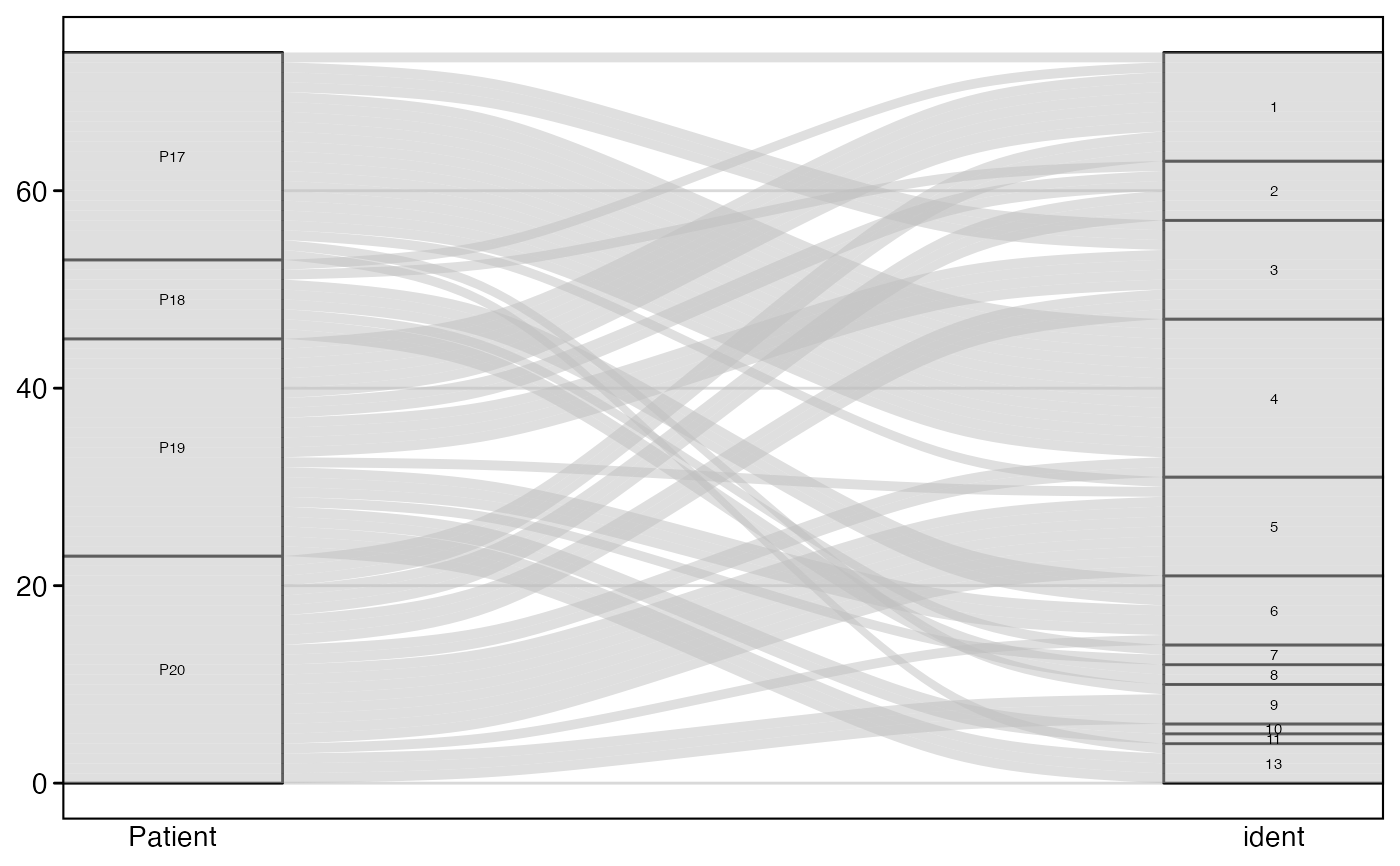
# Show only top 50 most frequent clones
alluvialClones(scRep_example,
                   clone.call = "aa",
                   y.axes = c("Patient", "ident"),
                   top.clones = 50)


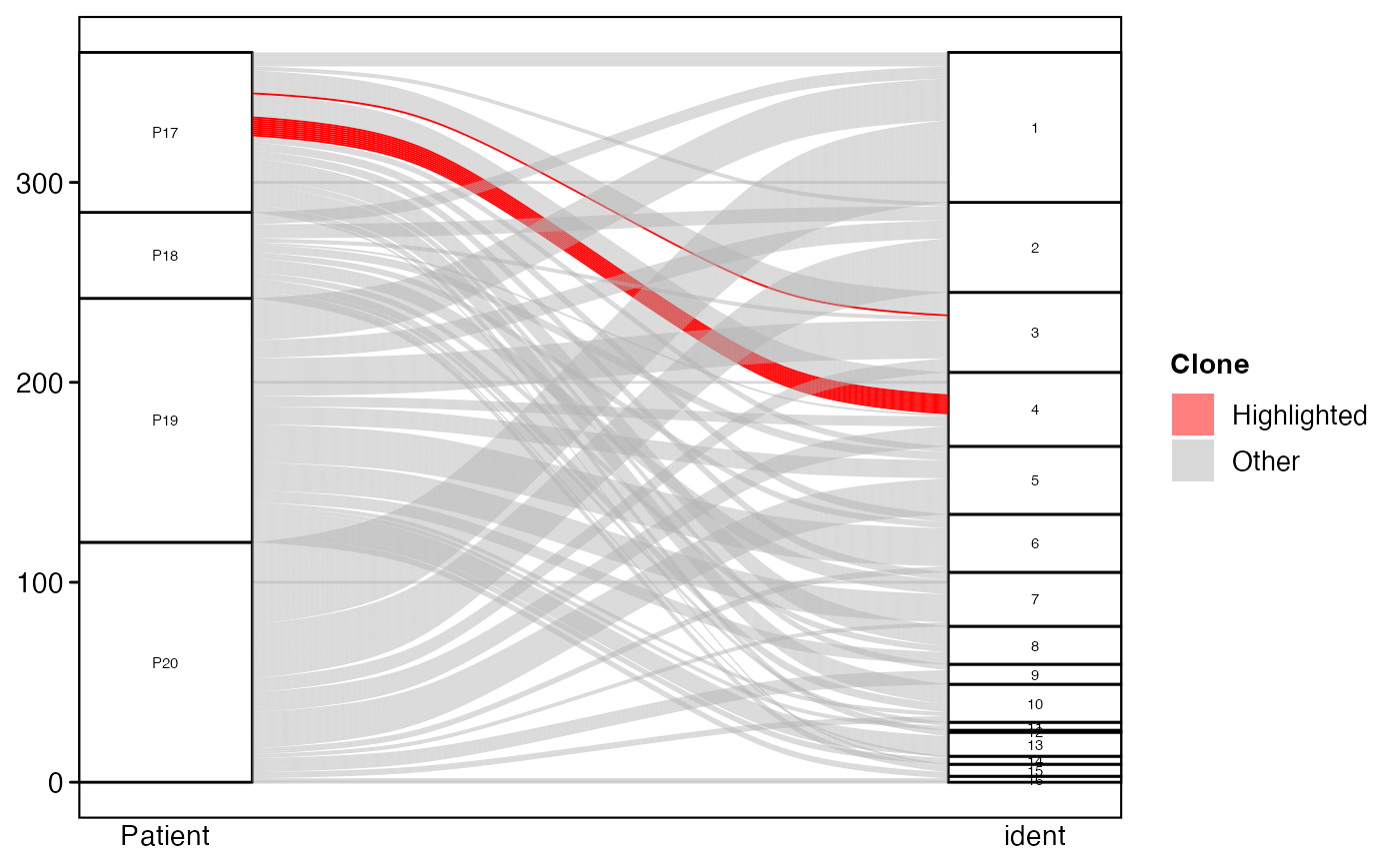
# Highlight specific clones
alluvialClones(scRep_example,
                   clone.call = "aa",
                   y.axes = c("Patient", "ident"),
                   highlight.clones = c("CVVSDNTGGFKTIF_CASSVRRERANTGELFF"))
#> Warning: Use of `lodes[[".highlight"]]` is discouraged.
#> ℹ Use `.data[[".highlight"]]` instead.
#> Warning: Use of `lodes[[".highlight"]]` is discouraged.
#> ℹ Use `.data[[".highlight"]]` instead.