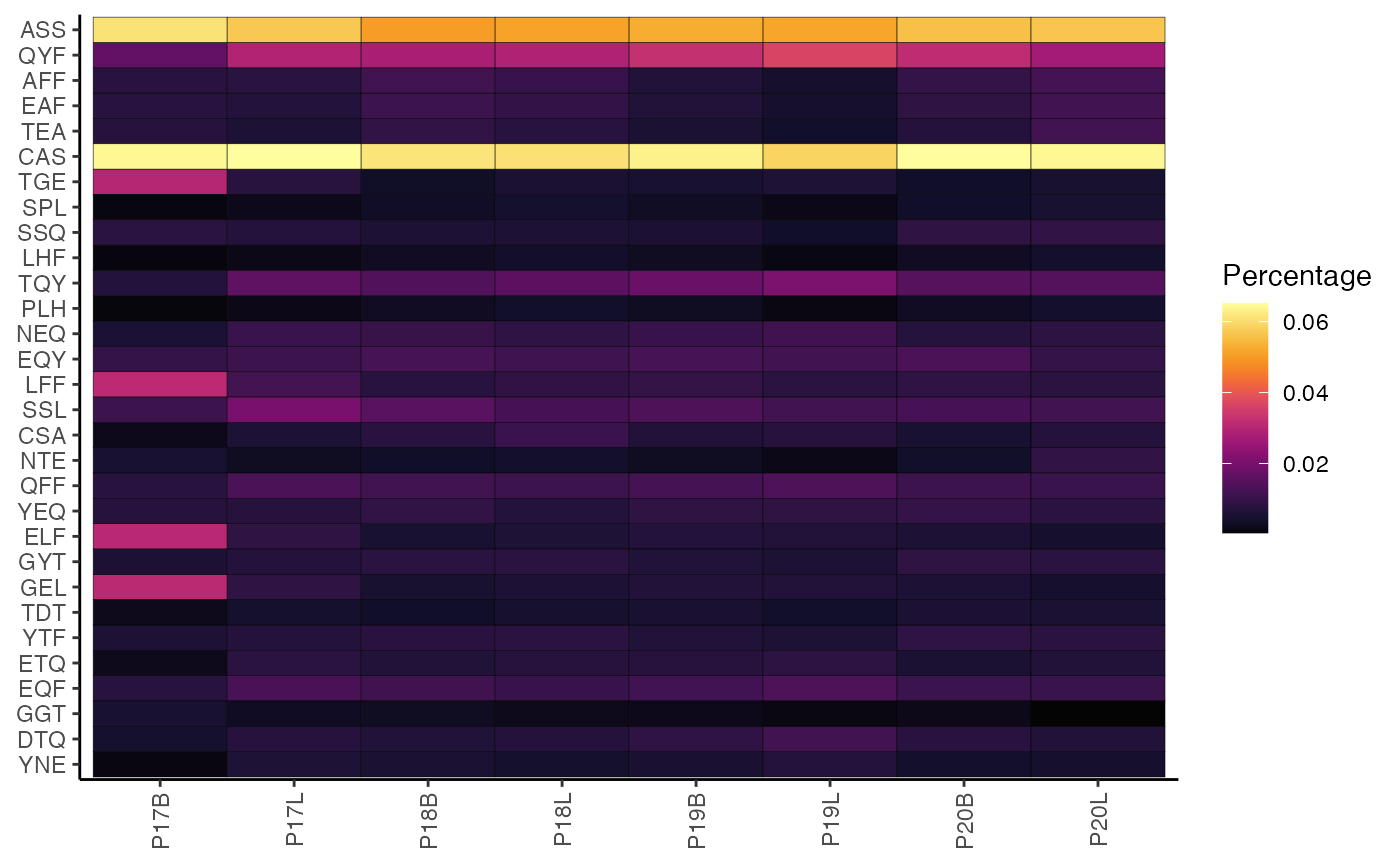
Analyze K-mer Motif Composition — percentKmer • scRepertoire

This function calculates and visualizes the frequency of k-mer motifs for either nucleotide (nt) or amino acid (aa) sequences. It produces a heatmap showing the relative composition of the most variable motifs across samples or groups.

percentKmer(
  input.data,
  chain = "TRB",
  cloneCall = "aa",
  group.by = NULL,
  order.by = NULL,
  motif.length = 3,
  min.depth = 3,
  top.motifs = 30,
  exportTable = FALSE,
  palette = "inferno",
  ...
)

Arguments

input.data: The product of combineTCR(), combineBCR(), or combineExpression()
chain: The TCR/BCR chain to use. Accepted values: TRA, TRB, TRG, TRD, IGH, or IGL (for both light chains).
cloneCall: Defines the clonal sequence grouping. Accepted values are: nt (CDR3 nucleotide sequence) or aa (CDR3 amino acid sequence).
group.by: A column header in the metadata or lists to group the analysis by (e.g., "sample", "treatment"). If NULL, data will be analyzed as by list element or active identity in the case of single-cell objects.
order.by: A character vector defining the desired order of elements of the group.by variable. Alternatively, use alphanumeric to sort groups automatically.
motif.length: The length of the kmer to analyze
min.depth: Minimum count a motif must reach to be retained in the output (>= 1). Default: 3.
top.motifs: Return the n most variable motifs as a function of median absolute deviation
exportTable: If TRUE, returns a data frame or matrix of the results instead of a plot.
palette: Colors to use in visualization - input any hcl.pals
...: Additional arguments passed to the ggplot theme

Value

A ggplot object displaying a heatmap of motif percentages. If exportTable = TRUE, a matrix of the raw data is returned.

Details

The function first calculates k-mer frequencies for each sample/group. By default, it then identifies the 30 most variable motifs based on the Median Absolute Deviation (MAD) across all samples and displays their frequencies in a heatmap.

Examples

# Making combined contig data
combined <- combineTCR(contig_list, 
                        samples = c("P17B", "P17L", "P18B", "P18L", 
                                    "P19B","P19L", "P20B", "P20L"))

# Using percentKmer()
percentKmer(combined, 
            chain = "TRB", 
            motif.length = 3)