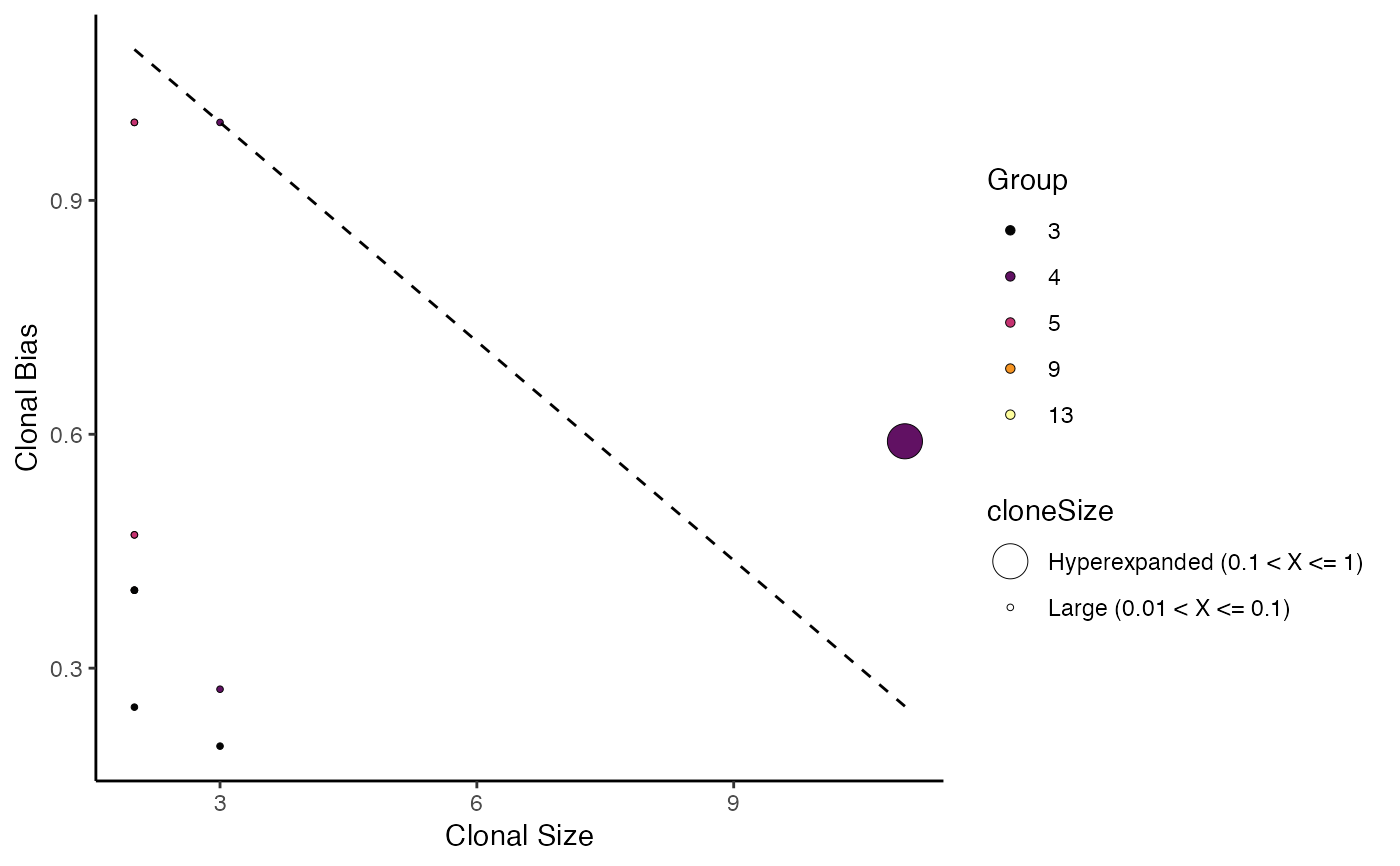
The metric seeks to quantify how individual clones are skewed towards
a specific cellular compartment or cluster. A clone bias of 1 -
indicates that a clone is composed of cells from a single
compartment or cluster, while a clone bias of 0 - matches the
background subtype distribution. Please read and cite the following
manuscript
if using clonalBias().
Usage
clonalBias(
  sc.data,
  clone.call = NULL,
  split.by = NULL,
  group.by = NULL,
  n.boots = 20,
  min.expand = 10,
  export.table = NULL,
  palette = "inferno",
  cloneCall = NULL,
  exportTable = NULL,
  ...
)
Arguments
- sc.data
The single-cell object after
combineExpression().- clone.call
Defines the clonal sequence grouping. Accepted values are:
gene(VDJC genes),nt(CDR3 nucleotide sequence),aa(CDR3 amino acid sequence), orstrict(VDJC + nt). A custom column header can also be used.- split.by
The variable to use for calculating the baseline frequencies. For example, "Type" for lung vs peripheral blood comparison
- group.by
A column header in the metadata that bias will be based on.
- n.boots
number of bootstraps to downsample.
- min.expand
clone frequency cut off for the purpose of comparison.
- export.table
If
TRUE, returns a data frame or matrix of the results instead of a plot.- palette
Colors to use in visualization - input any hcl.pals.
- cloneCall
![[Deprecated]](figures/lifecycle-deprecated.svg) Use
Use clone.callinstead.- exportTable
- Use
export.tableinstead. - ...
Additional arguments passed to the ggplot theme
Examples
# Making combined contig data
combined <- combineTCR(contig_list,
                        samples = c("P17B", "P17L", "P18B", "P18L",
                                    "P19B","P19L", "P20B", "P20L"))

# Getting a sample of a Seurat object
scRep_example <- get(data("scRep_example"))

# Using combineExpresion()
scRep_example <- combineExpression(combined, scRep_example)
scRep_example$Patient <- substring(scRep_example$orig.ident,1,3)

# Using clonalBias()
clonalBias(scRep_example,
              clone.call = "aa",
              split.by = "Patient",
              group.by = "seurat_clusters",
              n.boots = 5,
              min.expand = 2)
#> Smoothing formula not specified. Using: y ~ qss(x, lambda = 3)