Antibody Visualization
Nick Borcherding
Washington University in St. Louis, School of Medicine, St. Louis, MO, USACompiled: January 27, 2026
Source:vignettes/antibody-visualization.Rmd
antibody-visualization.RmdIntroduction
Visualizing HLA antibody data is essential for:
- Monitoring patient sensitization
- Identifying unacceptable antigens for transplant
- Tracking antibody trends over time
- Analyzing eplet-level reactivity patterns
This article covers deepMatchR’s visualization tools for Single Antigen Bead (SAB) and Panel Reactive Antibody (PRA) assay results.
Example Data
deepMatchR includes simulated assay data for demonstrations:
data("deepMatchR_example")

# Available datasets:
# 1. Class I SAB
# 2. Class II SAB
# 3. PRA

head(deepMatchR_example[[1]], 5)
#>   BeadID         SpecAbbr       Specificity NormalValue  RawData CountValue
#> 1      1  -,-,-,-,-,-,-,-       -,-,-,-,-,-          NA    48.04         77
#> 2      2  -,-,-,-,-,-,-,-       -,-,-,-,-,-          NA 14068.42         78
#> 3      3 A1,-,-,-,-,-,-,- A*01:01,-,-,-,-,-        0.00    37.41         73
#> 4      4 A2,-,-,-,-,-,-,- A*02:01,-,-,-,-,-      153.63   215.17         60
#> 5 5 A2,-,-,-,-,-,-,- A*02:03,-,-,-,-,- 127.24 180.22 85Plotting Antibodies
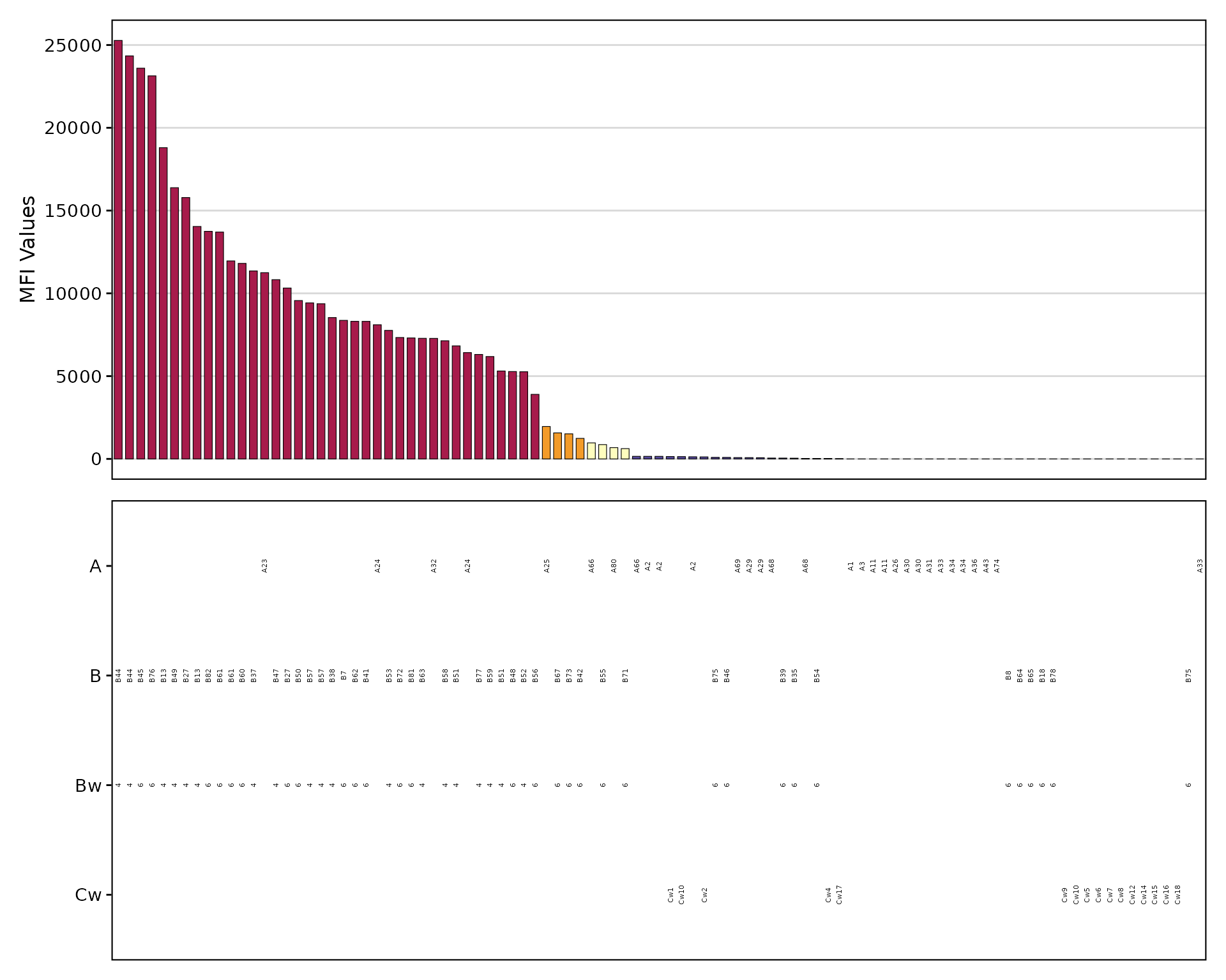
SAB Bar Plot
The plotAntibodies() function creates
publication-quality visualizations:
plotAntibodies(
  result_file = deepMatchR_example[[1]],
  type = "SAB",
  bead_cutoffs = c(2000, 1000, 500, 250),
  add_table = TRUE,
  palette = "spectral"
)
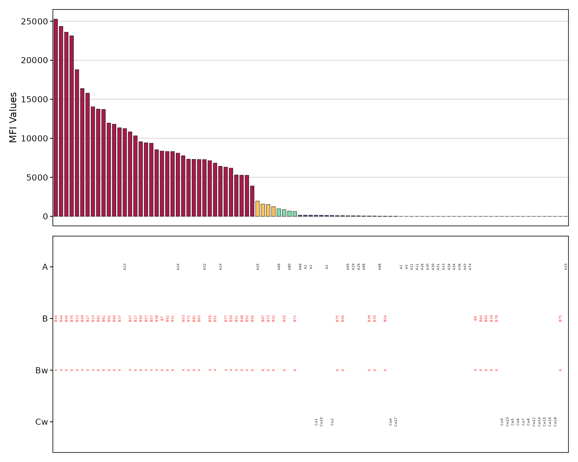
Highlighting Specific Antigens
Focus on antigens of interest using
highlight_antigen:
plotAntibodies(
  result_file = deepMatchR_example[[1]],
  type = "SAB",
  bead_cutoffs = c(2000, 1000, 500),
  add_table = TRUE,
  palette = "spectral",
  highlight_antigen = c("Bw4", "Bw6")
)
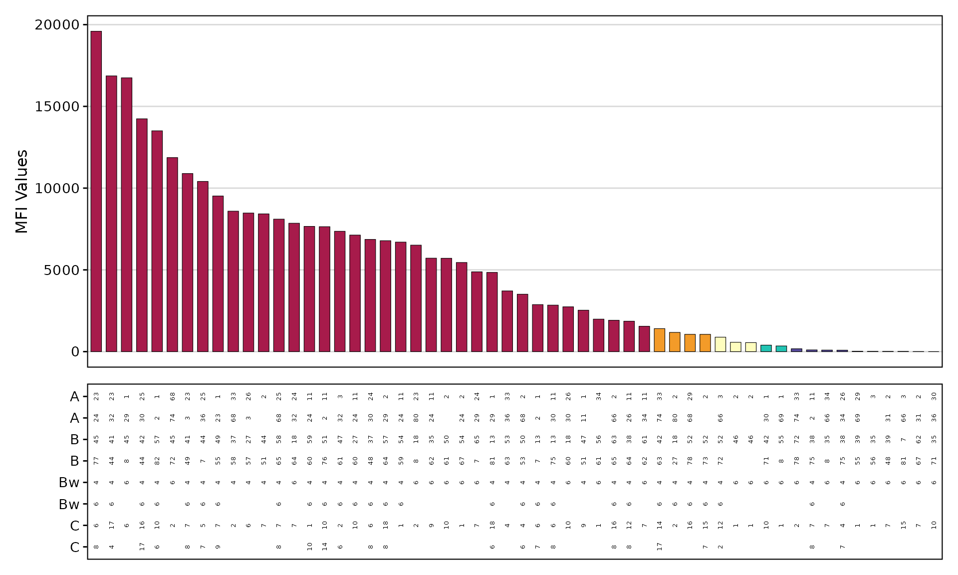
PRA Bar Plot
plotAntibodies(
  result_file = deepMatchR_example[[3]],
  type = "PRA",
  class = "I",
  add_table = TRUE,
  palette = "spectral"
)
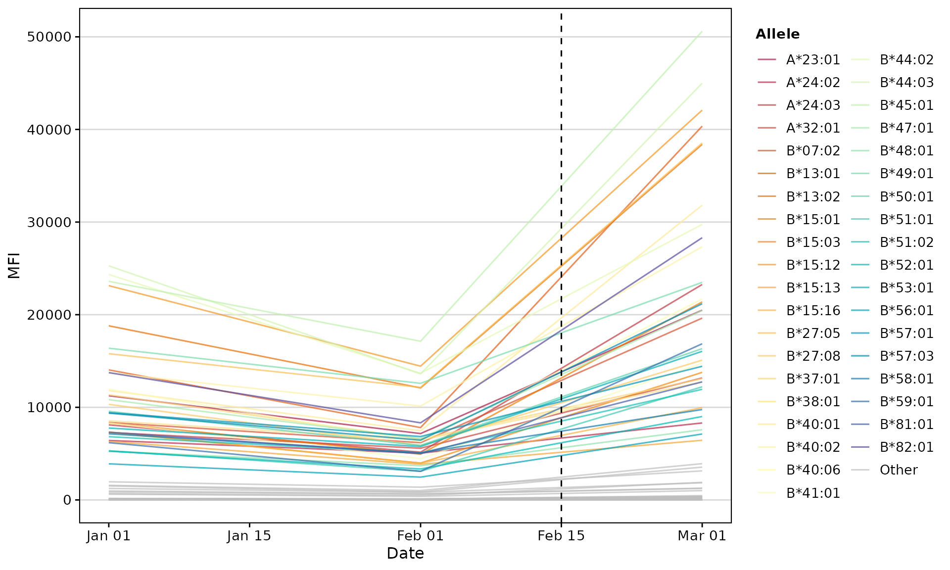
Time-Series Trend Plot
Track antibody levels over multiple time points:
# Simulate longitudinal data
set.seed(123)
sab_data_list <- list(
  "01/01/2023" = deepMatchR_example[[1]],
  "02/01/2023" = deepMatchR_example[[1]] %>%
    mutate(NormalValue = NormalValue * runif(n(), 0.5, 0.8)),
  "03/01/2023" = deepMatchR_example[[1]] %>%
    mutate(NormalValue = NormalValue * runif(n(), 1, 3))
)

plotAntibodies(
  result_file = sab_data_list,
  type = "SAB",
  plot_trend = TRUE,
  highlight_threshold = 5000,
  vline_dates = c("2023-02-15")
)
Eplet Visualization
plotEplets() Overview
The plotEplets() function offers three visualization
types:
| Type | Best For |
|---|---|
treemap |
Overview of eplet prominence |
bar |
Ranking eplets by positivity |
AUC |
Performance across thresholds |
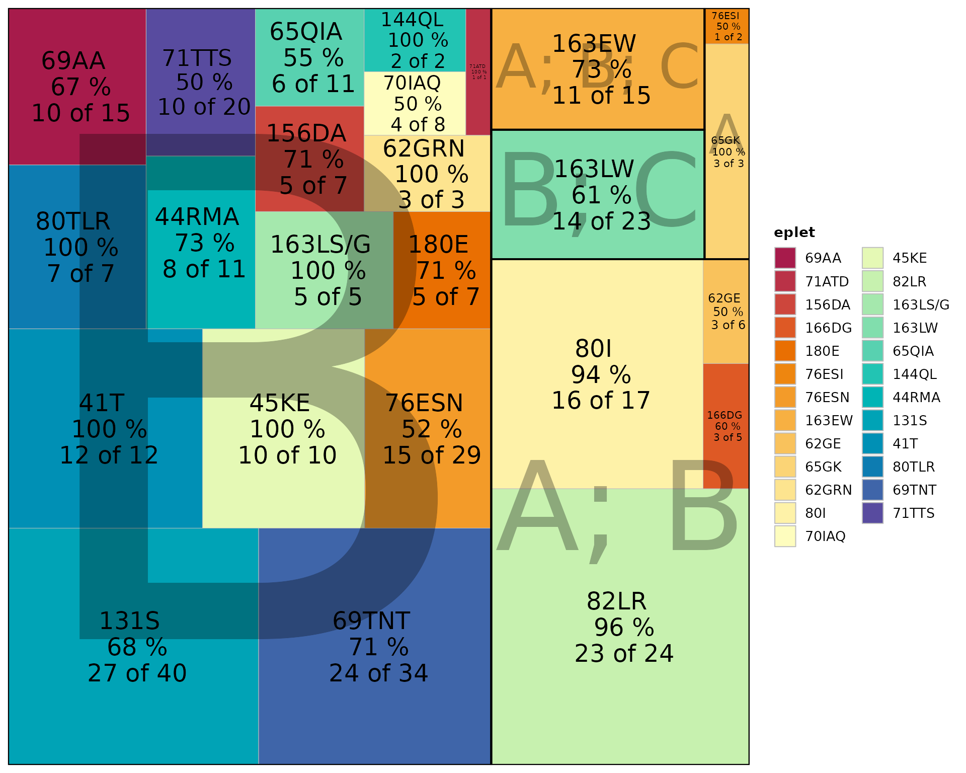
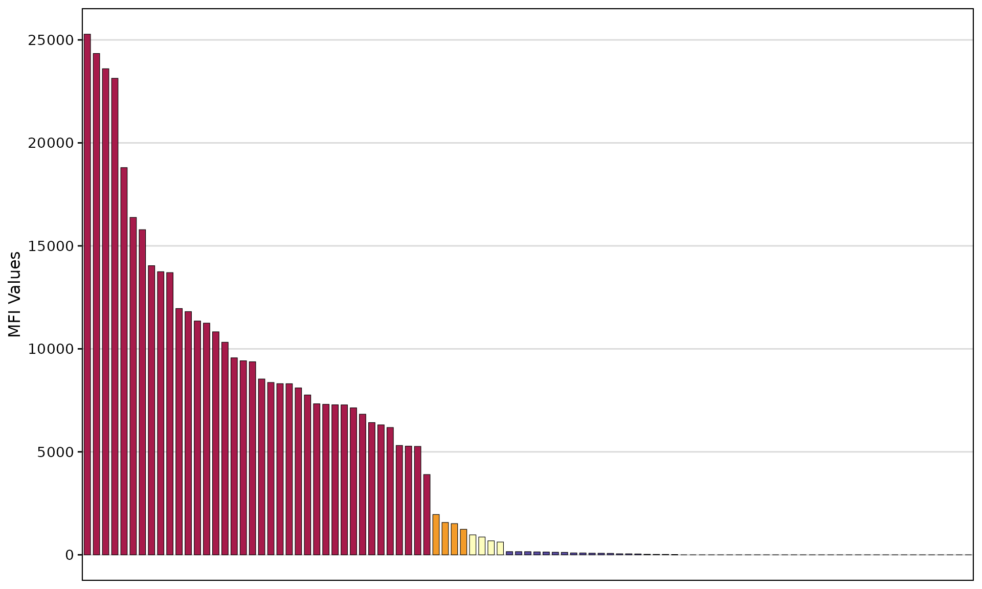
Treemap View
Tile area represents importance (positive beads × positivity rate):
plotEplets(
  result_file = deepMatchR_example[[1]],
  plot_type = "treemap",
  cutoff = 2000,
  evidence_level = c("A1", "A2", "B"),
  percPos_filter = 0.4,
  palette = "spectral"
)
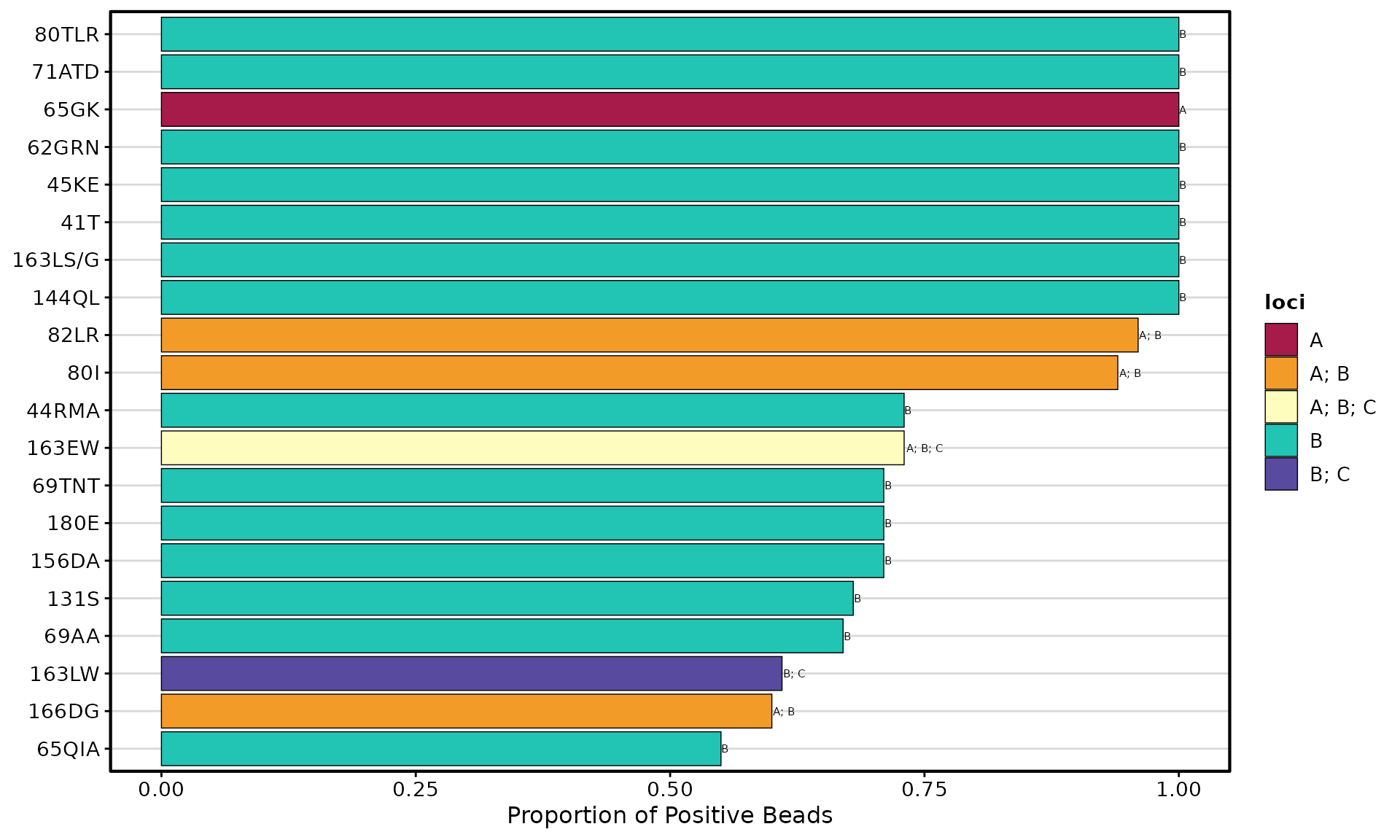
Bar Plot
Ranks eplets by positivity rate at a specific threshold:
plotEplets(
  result_file = deepMatchR_example[[1]],
  plot_type = "bar",
  group_by = "loci",
  cutoff = 2000,
  evidence_level = c("A1", "A2", "B"),
  percPos_filter = 0.4,
  top_eplets = 20,
  palette = "spectral"
)
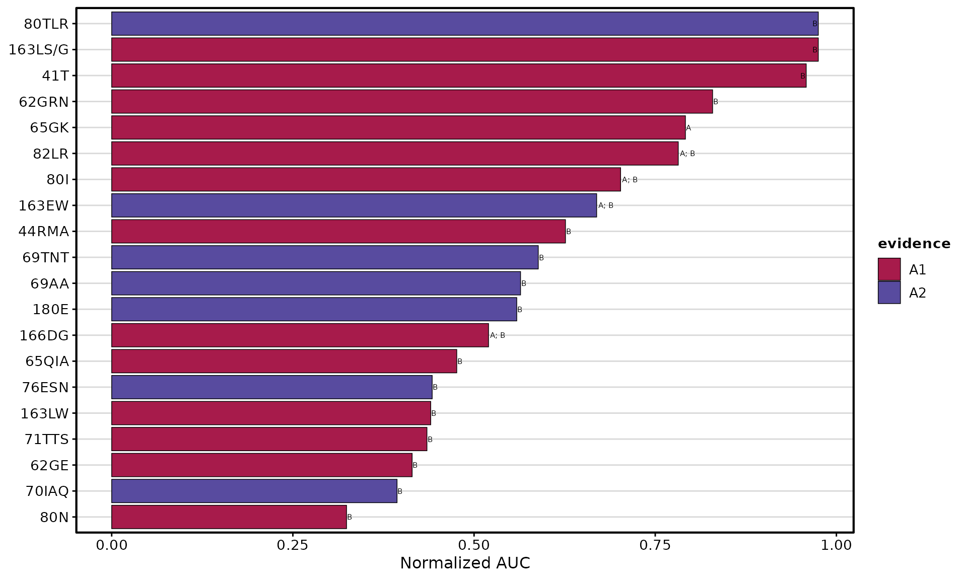
AUC Bar Plot
Ranks eplets by performance across multiple thresholds:
plotEplets(
  result_file = deepMatchR_example[[1]],
  plot_type = "AUC",
  percPos_filter = 0.4,
  group_by = "evidence_level",
  cut_min = 250,
  cut_max = 10000,
  cut_step = 250,
  top_eplets = 20,
  palette = "spectral"
)
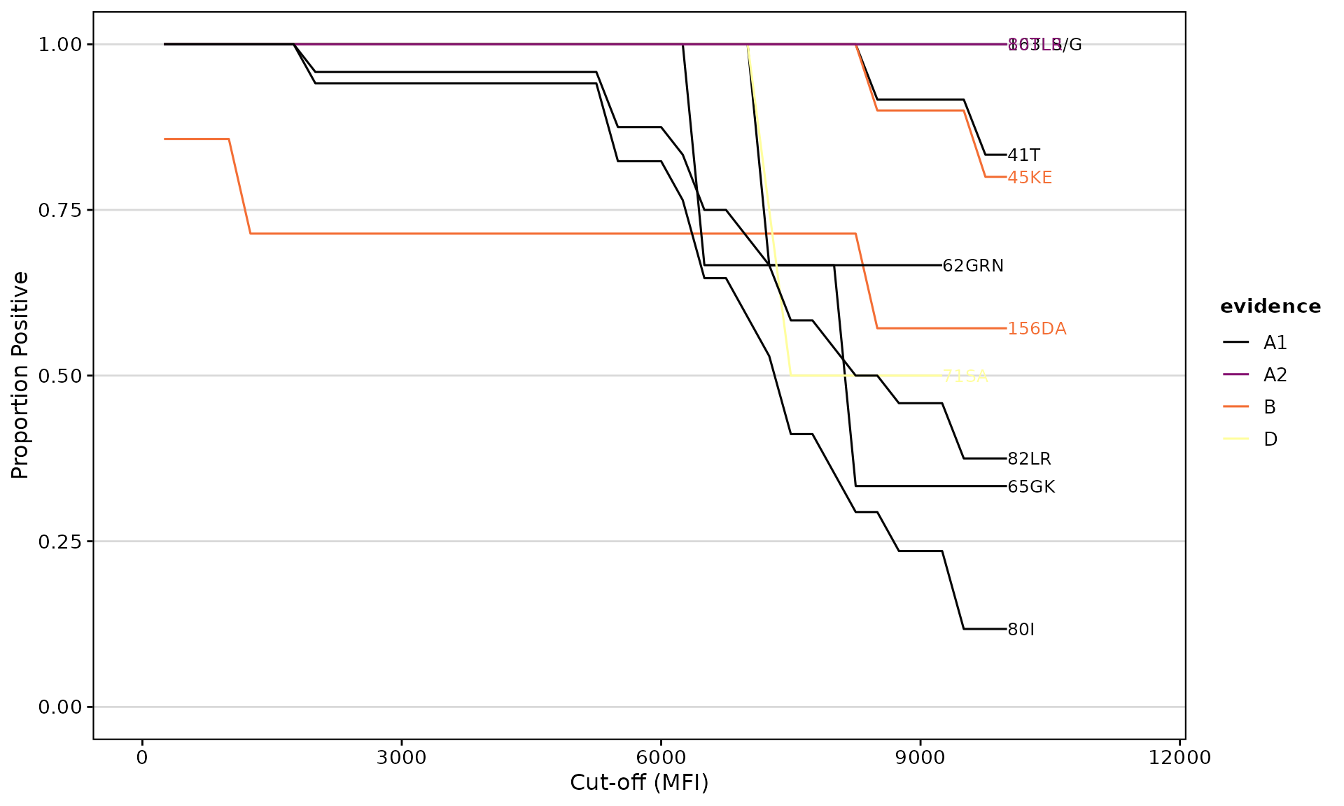
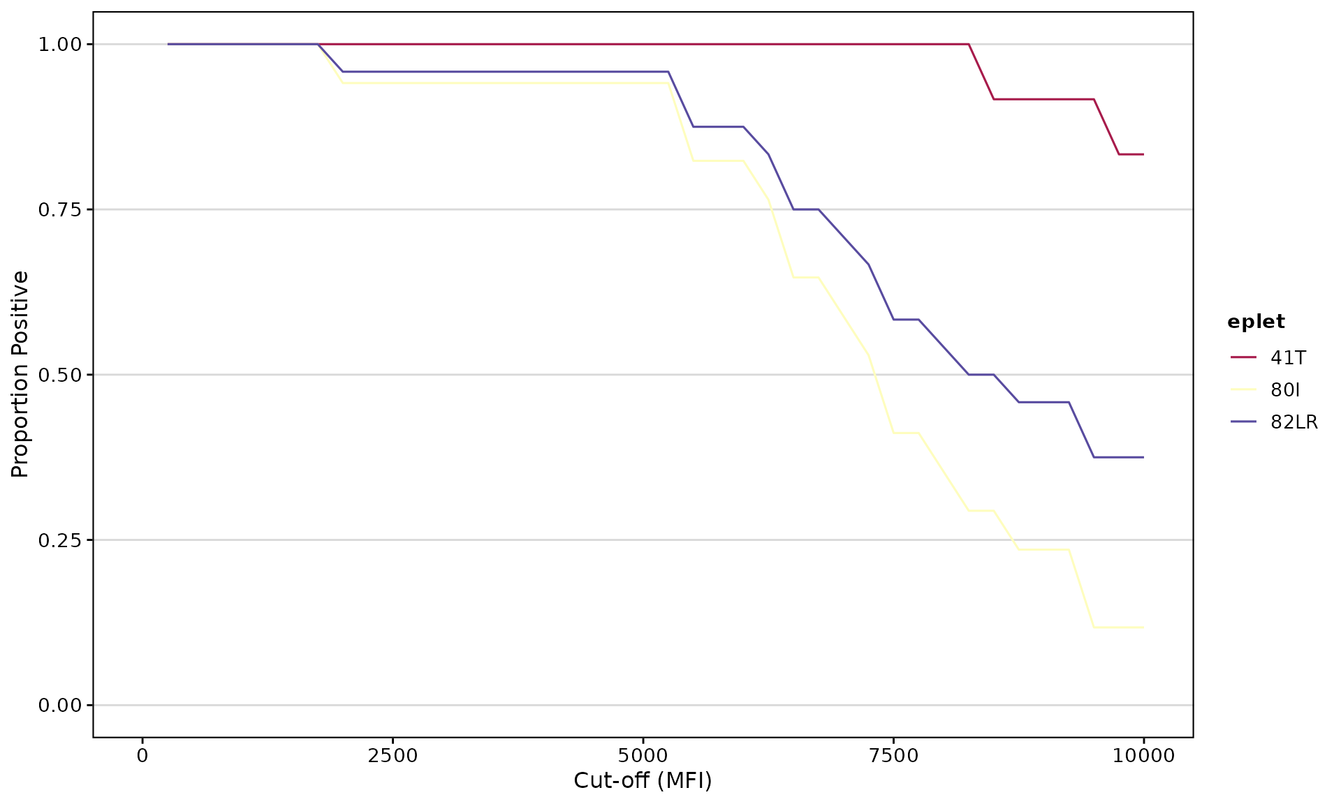
Eplet AUC Analysis
epletAUC() Function
Calculates the Area Under the Curve for eplet reactivity across multiple MFI thresholds. This provides a more robust measure than a single cutoff.
Visualize Reactivity Curves
epletAUC(
  result_file = deepMatchR_example[[1]],
  group_by = "evidence",
  evidence_level = c("A1", "A2", "B", "D"),
  plot_results = TRUE,
  cut_min = 250,
  cut_max = 10000,
  cut_step = 250,
  palette = "inferno"
)
Get AUC Values as Data
auc_result <- epletAUC(
  result_file = deepMatchR_example[[1]],
  plot_results = FALSE,
  cut_min = 250,
  cut_max = 10000,
  cut_step = 250
)
head(auc_result)
#>     eplet      AUC total_count   loci  norm_AUC
#>    <char>    <num>       <int> <char>     <num>
#> 1:   82LR 7817.708          24   A; B 0.7817708
#> 2:    80I 7022.059          17   A; B 0.7022059
#> 3:   69AA 5641.667          15      B 0.5641667
#> 4:  163EW 6691.667          15   A; B 0.6691667
#> 5:    41T 9583.333          12      B 0.9583333
#> 6:  65QIA 4761.364          11      B 0.4761364
Advanced Filtering
epletAUC(
  result_file = deepMatchR_example[[1]],
  label = FALSE,
  plot_results = TRUE,
  eplet_filter = 10,      # Minimum bead count
  percPos_filter = 1.0    # Minimum positivity threshold
)
Customization Options
Color Palettes
Available palettes include:
-
spectral- Rainbow diverging -
inferno- Yellow to purple -
viridis- Green to purple -
plasma- Yellow to magenta
# Using inferno palette
plotEplets(
  result_file = deepMatchR_example[[1]],
  plot_type = "bar",
  cutoff = 2000,
  top_eplets = 15,
  palette = "inferno"
)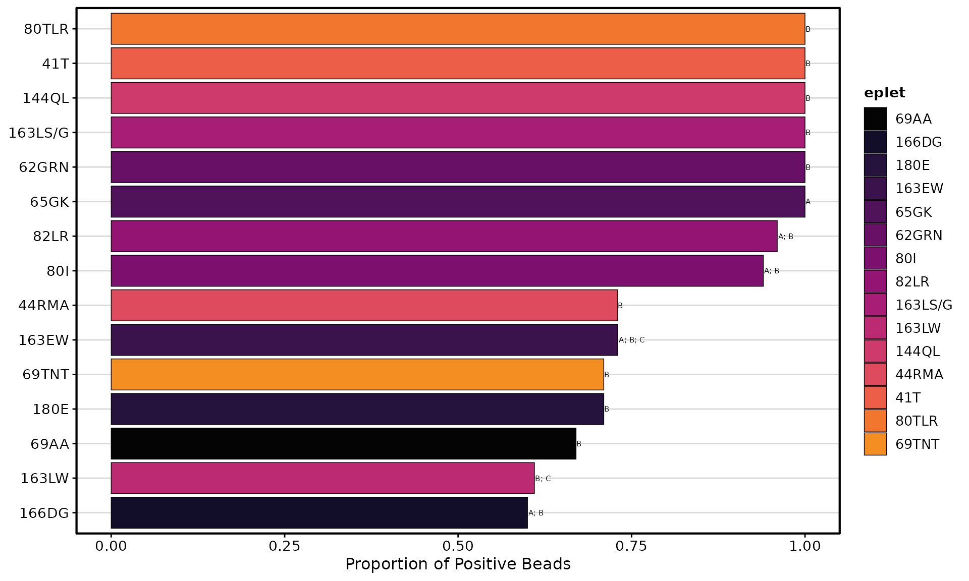
Table Options
Control the summary table with add_table:
# Without table
plotAntibodies(
  result_file = deepMatchR_example[[1]],
  type = "SAB",
  add_table = FALSE
)
Function Reference
plotAntibodies()
| Argument | Default | Description |
|---|---|---|
result_file |
– | SAB/PRA data frame or named list for trends |
type |
"SAB" |
Assay type: “SAB” or “PRA” |
class |
NULL |
HLA class filter: “I” or “II” |
bead_cutoffs |
c(2000,1000,500,250) |
MFI cutoff thresholds |
add_table |
TRUE |
Include summary table |
palette |
"spectral" |
Color palette |
highlight_antigen |
NULL |
Antigens to highlight |
plot_trend |
FALSE |
Create time-series plot |
vline_dates |
NULL |
Vertical line dates for trends |
plotEplets()
| Argument | Default | Description |
|---|---|---|
result_file |
– | SAB data frame |
plot_type |
"treemap" |
“treemap”, “bar”, or “AUC” |
cutoff |
2000 |
MFI cutoff for positive |
evidence_level |
c("A1","A2","B") |
Evidence levels to include |
percPos_filter |
0.4 |
Minimum positivity rate |
top_eplets |
20 |
Number of top eplets for bar plots |
group_by |
"evidence" |
Grouping variable |
palette |
"spectral" |
Color palette |
epletAUC()
| Argument | Default | Description |
|---|---|---|
result_file |
– | SAB data frame |
plot_results |
TRUE |
Generate plot |
cut_min, cut_max
|
250, 10000
|
MFI range |
cut_step |
250 |
Step size |
eplet_filter |
NULL |
Minimum bead count |
percPos_filter |
NULL |
Minimum final positivity |
label |
TRUE |
Add labels to plot |
palette |
"spectral" |
Color palette |
Session Information
sessionInfo()
#> R version 4.5.2 (2025-10-31)
#> Platform: x86_64-pc-linux-gnu
#> Running under: Ubuntu 24.04.3 LTS
#>
#> Matrix products: default
#> BLAS:   /usr/lib/x86_64-linux-gnu/openblas-pthread/libblas.so.3
#> LAPACK: /usr/lib/x86_64-linux-gnu/openblas-pthread/libopenblasp-r0.3.26.so;  LAPACK version 3.12.0
#>
#> locale:
#>  [1] LC_CTYPE=C.UTF-8       LC_NUMERIC=C           LC_TIME=C.UTF-8
#>  [4] LC_COLLATE=C.UTF-8     LC_MONETARY=C.UTF-8    LC_MESSAGES=C.UTF-8
#>  [7] LC_PAPER=C.UTF-8       LC_NAME=C              LC_ADDRESS=C
#> [10] LC_TELEPHONE=C         LC_MEASUREMENT=C.UTF-8 LC_IDENTIFICATION=C
#>
#> time zone: UTC
#> tzcode source: system (glibc)
#>
#> attached base packages:
#> [1] stats     graphics  grDevices utils     datasets  methods   base
#>
#> other attached packages:
#> [1] ggplot2_4.0.1     dplyr_1.1.4       deepMatchR_0.99.0 BiocStyle_2.38.0
#>
#> loaded via a namespace (and not attached):
#>  [1] ggfittext_0.10.3       gtable_0.3.6           dir.expiry_1.18.0
#>  [4] xfun_0.56              bslib_0.10.0           lattice_0.22-7
#>  [7] quadprog_1.5-8         vctrs_0.7.1            tools_4.5.2
#> [10] generics_0.1.4         stats4_4.5.2           parallel_4.5.2
#> [13] tibble_3.3.1           pkgconfig_2.0.3        Matrix_1.7-4
#> [16] data.table_1.18.0      RColorBrewer_1.1-3     S7_0.2.1
#> [19] desc_1.4.3             S4Vectors_0.48.0       readxl_1.4.5
#> [22] lifecycle_1.0.5        compiler_4.5.2         farver_2.1.2
#> [25] textshaping_1.0.4      Biostrings_2.78.0      Seqinfo_1.0.0
#> [28] htmltools_0.5.9        sass_0.4.10            yaml_2.3.12
#> [31] pillar_1.11.1          pkgdown_2.2.0          crayon_1.5.3
#> [34] jquerylib_0.1.4        cachem_1.1.0           basilisk_1.22.0
#> [37] tidyselect_1.2.1       rvest_1.0.5            digest_0.6.39
#> [40] stringi_1.8.7          bookdown_0.46          labeling_0.4.3
#> [43] fastmap_1.2.0          grid_4.5.2             treemapify_2.6.0
#> [46] cli_3.6.5              magrittr_2.0.4         patchwork_1.3.2
#> [49] withr_3.0.2            filelock_1.0.3         scales_1.4.0
#> [52] rmarkdown_2.30         pwalign_1.6.0          XVector_0.50.0
#> [55] httr_1.4.7             reticulate_1.44.1      cellranger_1.1.0
#> [58] ragg_1.5.0             png_0.1-8              memoise_2.0.1
#> [61] evaluate_1.0.5         knitr_1.51             IRanges_2.44.0
#> [64] immReferent_0.99.6     rlang_1.1.7            Rcpp_1.1.1
#> [67] glue_1.8.0             BiocManager_1.30.27    xml2_1.5.2
#> [70] directlabels_2025.6.24 BiocGenerics_0.56.0    svglite_2.2.2
#> [73] jsonlite_2.0.0         R6_2.6.1               systemfonts_1.3.1
#> [76] fs_1.6.6