Advanced Tuning & Workflows

Introduction

This vignette covers advanced usage patterns for bHIVE:

Hyperparameter tuning with swarmbHIVE() across tasks
Multilayer hierarchical refinement with honeycombHIVE()
Gradient-based prototype refinement with refineB()
Integration with the caret framework
Visualization with visualizeHIVE()

Hyperparameter Tuning with swarmbHIVE

swarmbHIVE() performs grid search over bHIVE hyperparameters and evaluates each combination using a task-specific metric.

Available Metrics

Task	Metrics	Direction
Clustering	`"silhouette"`, `"davies_bouldin"`, `"calinski_harabasz"`	Higher is better (except D-B)
Classification	`"accuracy"`, `"balanced_accuracy"`, `"f1"`, `"kappa"`	Higher is better

Clustering Tuning

data(iris)
X <- as.matrix(iris[, 1:4])

grid <- expand.grid(
  nAntibodies = c(10, 20, 30),
  beta        = c(3, 5),
  epsilon     = c(0.01, 0.05)
)

set.seed(42)
tuning <- swarmbHIVE(X = X, task = "clustering", grid = grid,
                     metric = "silhouette", maxIter = 15, verbose = FALSE)

ggplot(tuning$results, aes(x = nAntibodies, y = metric_value,
                            color = factor(beta))) +
  geom_line() +
  geom_point(aes(shape = factor(epsilon)), size = 3) +
  labs(title = "Clustering: Silhouette Score",
       x = "Number of Antibodies", y = "Silhouette",
       color = "Beta", shape = "Epsilon") +
  scale_color_viridis(discrete = TRUE) +
  theme_minimal()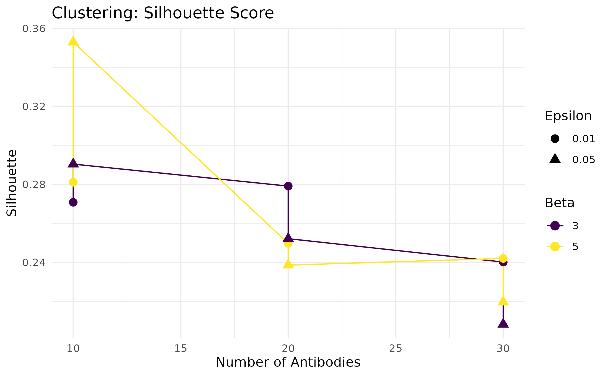

tuning$best_params

##    nAntibodies beta epsilon metric_value
## 10          10    5    0.05    0.3529172

Classification Tuning

y <- iris$Species
grid_cls <- expand.grid(
  nAntibodies = c(15, 30, 50),
  beta        = c(3, 5, 10),
  epsilon     = c(0.01, 0.05)
)

set.seed(42)
tuning_cls <- swarmbHIVE(X = X, y = y, task = "classification",
                         grid = grid_cls, metric = "accuracy",
                         maxIter = 15, verbose = FALSE)
tuning_cls$best_params

##    nAntibodies beta epsilon metric_value
## 11          30    3    0.05    0.9733333

Parallelization with BiocParallel

swarmbHIVE() accepts a BPPARAM argument for parallel execution. This is especially useful when the grid is large:

library(BiocParallel)

# Use 4 cores
tuning <- swarmbHIVE(
  X = X, y = y, task = "classification",
  grid = grid_cls, metric = "accuracy",
  BPPARAM = MulticoreParam(4),
  verbose = FALSE
)

honeycombHIVE() runs bHIVE iteratively across multiple layers. Each layer produces prototypes that become the input for the next layer, creating a hierarchical compression of the data.

Basic Multilayer Clustering

set.seed(42)
res <- honeycombHIVE(X = X, task = "clustering",
                     layers = 3, nAntibodies = 30,
                     beta = 5, epsilon = 0.05,
                     maxIter = 10, verbose = FALSE)

# Each layer progressively refines cluster structure
layer_info <- sapply(res, function(r) {
  c(n_prototypes = nrow(r$antibodies),
    n_clusters = length(unique(r$membership)))
})
layer_info

##              [,1] [,2] [,3]
## n_prototypes   27   15   10
## n_clusters     27   15   10

Collapse Methods

The collapseMethod parameter controls how clusters are summarized into prototypes for the next layer:

Method	Description
`"centroid"`	Mean of cluster members (default)
`"medoid"`	Actual data point closest to center
`"median"`	Coordinate-wise median

set.seed(42)
res_centroid <- honeycombHIVE(X = X, task = "clustering", layers = 2,
                              nAntibodies = 20, collapseMethod = "centroid",
                              verbose = FALSE)
res_medoid <- honeycombHIVE(X = X, task = "clustering", layers = 2,
                            nAntibodies = 20, collapseMethod = "medoid",
                            verbose = FALSE)

cat("Centroid clusters:", length(unique(res_centroid[[2]]$membership)), "\n")

## Centroid clusters: 11

cat("Medoid clusters:  ", length(unique(res_medoid[[2]]$membership)), "\n")

## Medoid clusters:   13

Setting refine = TRUE applies gradient-based updates via refineB() after each layer’s bHIVE pass. This fine-tunes prototype positions before collapsing.

data(iris)
X_iris <- as.matrix(iris[, 1:4])
y_iris <- iris$Species

set.seed(42)
res_plain <- honeycombHIVE(X = X_iris, y = y_iris, task = "classification",
                           layers = 3, nAntibodies = 30, verbose = FALSE)

res_refined <- honeycombHIVE(X = X_iris, y = y_iris, task = "classification",
                             layers = 3, nAntibodies = 30,
                             refine = TRUE, refineOptimizer = "adam",
                             refineLoss = "categorical_crossentropy",
                             refineSteps = 5, refineLR = 0.01, verbose = FALSE)

acc_plain   <- mean(res_plain[[3]]$predictions   == as.character(y_iris))
acc_refined <- mean(res_refined[[3]]$predictions == as.character(y_iris))
cat("Accuracy (plain):  ", round(acc_plain, 3), "\n")

## Accuracy (plain):   0.333

cat("Accuracy (refined):", round(acc_refined, 3), "\n")

## Accuracy (refined): 0.333

refineB() takes trained antibody positions and fine-tunes them using gradient-based optimization. It supports 5 optimizers and 8 loss functions.

Optimizers

Optimizer	Key Parameter	Notes
`"sgd"`	`lr`	Simple, good baseline
`"momentum"`	`momentum_coef`	Accelerates SGD
`"adagrad"`	–	Per-parameter adaptive learning rates
`"adam"`	`beta1`, `beta2`	Best general-purpose optimizer
`"rmsprop"`	`rmsprop_decay`	Good for non-stationary objectives

Loss Functions

Loss	Tasks	Description
`"mae"`	All	Mean absolute error (sign-based pull/push)
`"categorical_crossentropy"`	Classification	Cross-entropy loss
`"binary_crossentropy"`	Classification	Binary cross-entropy
`"kullback_leibler"`	Classification	KL divergence
`"cosine"`	Classification	Cosine distance loss

Comparing Optimizers

X <- as.matrix(iris[, 1:4])
y <- iris$Species

set.seed(42)
res <- bHIVE(X, y, task = "classification", nAntibodies = 10,
             beta = 5, epsilon = 0.05, initMethod = "random",
             k = 4, verbose = FALSE)

Ab <- res$antibodies
colnames(Ab) <- colnames(X)
assignments <- as.integer(factor(res$assignments,
                                 levels = unique(res$assignments)))

pca <- prcomp(X, scale. = TRUE)
X_pca <- pca$x[, 1:2]
A_orig_pca <- predict(pca, Ab)

optimizers <- c("sgd", "adam", "rmsprop")
refined_list <- lapply(optimizers, function(opt) {
  Ab_refined <- refineB(A = Ab, X = X, y = y,
                        assignments = assignments,
                        task = "classification",
                        loss = "categorical_crossentropy",
                        optimizer = opt, steps = 5, lr = 0.01,
                        verbose = FALSE)
  colnames(Ab_refined) <- colnames(X)
  A_ref_pca <- predict(pca, Ab_refined)
  data.frame(optimizer = opt,
             PC1_after = A_ref_pca[, 1],
             PC2_after = A_ref_pca[, 2])
})

refined_df <- do.call(rbind, refined_list)
refined_df$ID <- factor(rep(seq_len(nrow(Ab)), times = length(optimizers)))

proto_df <- data.frame(ID = factor(seq_len(nrow(A_orig_pca))),
                       PC1_before = A_orig_pca[, 1],
                       PC2_before = A_orig_pca[, 2])

merged <- merge(proto_df, refined_df, by = "ID")

ggplot() +
  geom_point(data = data.frame(PC1 = X_pca[, 1], PC2 = X_pca[, 2],
                                Cluster = factor(assignments)),
             aes(x = PC1, y = PC2, color = Cluster), alpha = 0.4) +
  geom_point(data = proto_df,
             aes(x = PC1_before, y = PC2_before),
             color = "#440154", size = 4) +
  geom_point(data = merged,
             aes(x = PC1_after, y = PC2_after),
             color = "#FDE725", size = 4) +
  geom_segment(data = merged,
               aes(x = PC1_before, y = PC2_before,
                   xend = PC1_after, yend = PC2_after),
               arrow = arrow(length = unit(0.2, "cm"), type = "closed"),
               color = "black", linewidth = 0.5) +
  scale_color_viridis(discrete = TRUE) +
  labs(title = "Prototype Movement by Optimizer",
       subtitle = "Purple = before, Yellow = after refinement",
       x = "PC1", y = "PC2") +
  facet_wrap(~optimizer, nrow = 1,
             labeller = as_labeller(c(sgd = "SGD", adam = "Adam",
                                      rmsprop = "RMSProp"))) +
  theme_minimal()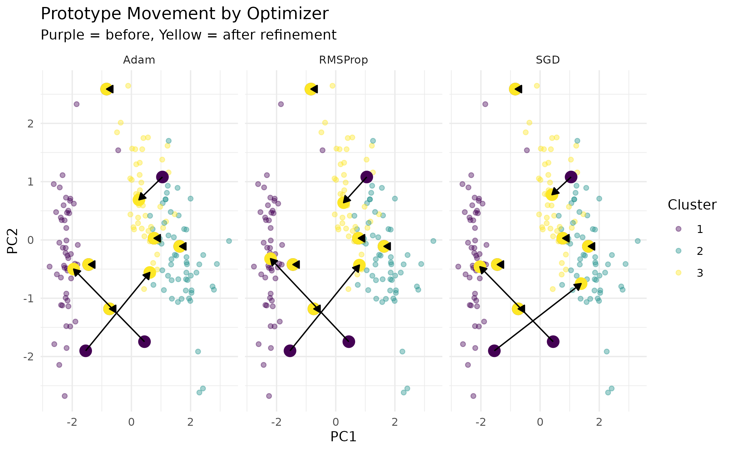

caret Integration

bHIVE provides two caret-compatible model objects for use with train():

bHIVEmodel – single-pass bHIVE with tuning over nAntibodies, beta, and epsilon
honeycombHIVEmodel – multilayer bHIVE with additional tuning over layers, refineOptimizer, refineSteps, and refineLR

Basic caret Workflow

library(caret)

data(iris)
X_iris <- as.matrix(iris[, 1:4])
y_iris <- iris$Species

set.seed(42)
idx <- sample(nrow(X_iris), nrow(X_iris) * 0.7)
X_train <- X_iris[idx, ]
X_test  <- X_iris[-idx, ]
y_train <- y_iris[idx]
y_test  <- y_iris[-idx]

ctrl <- trainControl(method = "cv", number = 3)

model <- train(
  x = X_train, y = y_train,
  method = bHIVEmodel,
  trControl = ctrl,
  tuneGrid = expand.grid(
    nAntibodies = c(10, 20),
    beta        = c(3, 5),
    epsilon     = c(0.01, 0.05)
  ),
  verbose = FALSE
)

ggplot(model) +
  labs(title = "caret Cross-Validation Results") +
  scale_color_viridis(discrete = TRUE) +
  theme_minimal()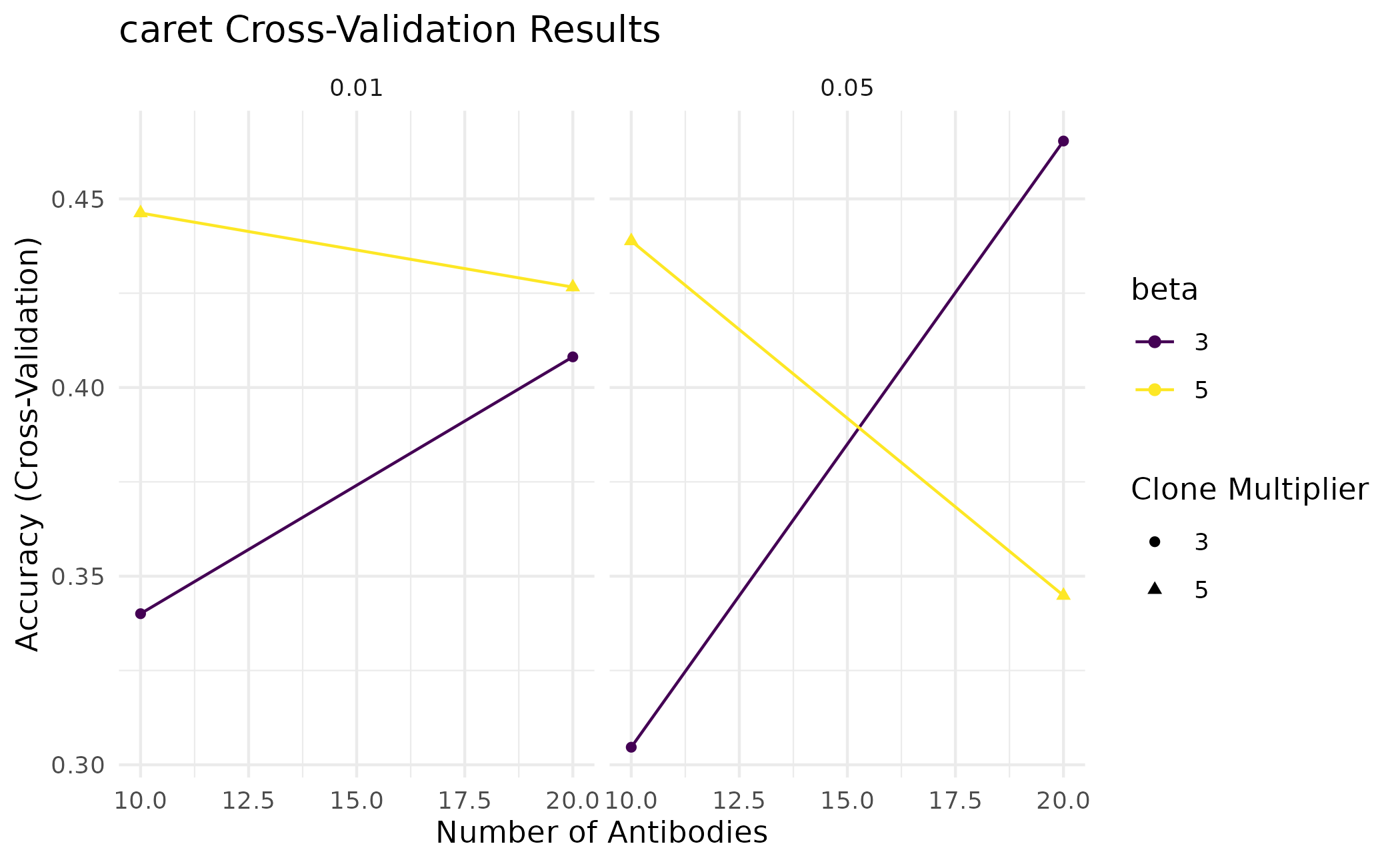

Prediction on Held-Out Data

preds <- predict(model, newdata = X_test)
table(Predicted = preds, Actual = y_test)

##             Actual
## Predicted    setosa versicolor virginica
##   setosa          0          6         7
##   versicolor      2          7         8
##   virginica      10          2         3

honeycombHIVE caret Model

The multilayer caret model adds layer count and refinement parameters to the tuning grid:

model_hc <- train(
  x = X_train, y = y_train,
  method = honeycombHIVEmodel,
  trControl = trainControl(method = "cv", number = 3),
  tuneGrid = expand.grid(
    nAntibodies = c(20, 30),
    beta        = 5,
    epsilon     = 0.05,
    layers      = c(2, 3),
    refineOptimizer = "adam",
    refineSteps     = 5,
    refineLR        = 0.01
  ),
  verbose = FALSE
)

Visualization with visualizeHIVE

The visualizeHIVE() function produces publication-ready ggplot2 figures for bHIVE and honeycombHIVE results.

Plot Types

Type	Description
`"scatter"`	2D scatter with optional dimensionality reduction (PCA, UMAP, t-SNE)
`"boxplot"`	Feature distributions by group with prototype overlay
`"violin"`	Violin plots with prototype markers
`"density"`	Density curves with prototype reference lines

Scatter Plot with PCA

X <- as.matrix(iris[, 1:4])

set.seed(42)
res <- honeycombHIVE(X = X, task = "clustering", layers = 3,
                     nAntibodies = 30, beta = 5, epsilon = 0.05,
                     maxIter = 10, verbose = FALSE)

visualizeHIVE(result = res, X = iris[, 1:4],
              plot_type = "scatter",
              transformation_method = "PCA",
              title = "Clustering (Layer 2)",
              layer = 2, task = "clustering")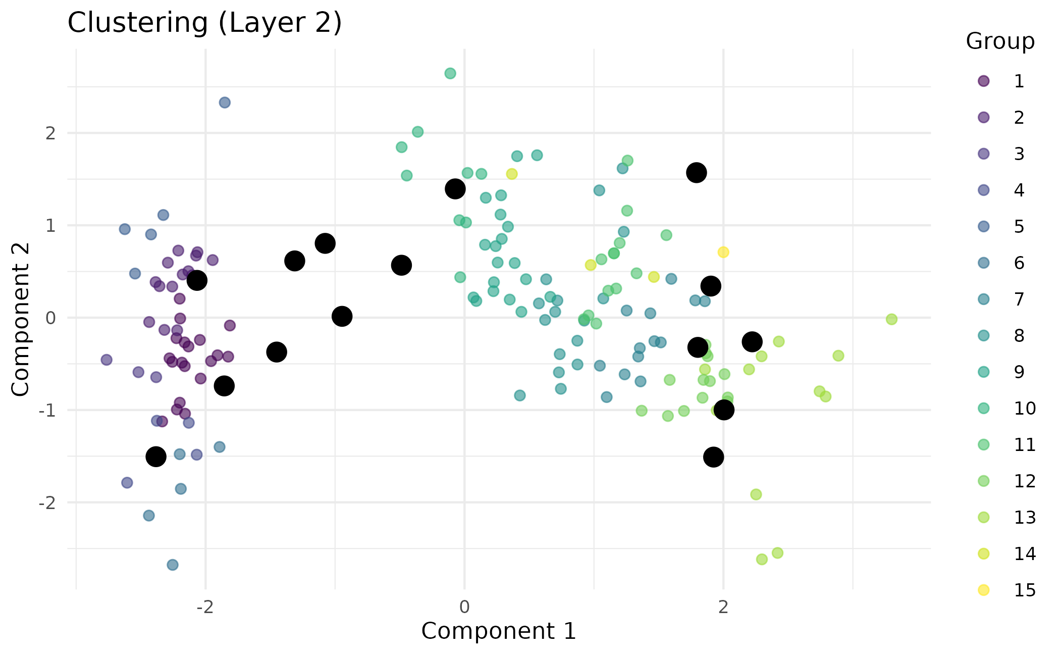

Violin Plot for Classification

set.seed(42)
res_cls <- honeycombHIVE(X = X, y = iris$Species,
                         task = "classification",
                         layers = 2, nAntibodies = 15,
                         beta = 5, maxIter = 10, verbose = FALSE)

visualizeHIVE(result = res_cls, X = iris[, 1:4],
              plot_type = "violin", feature = "Petal.Length",
              title = "Petal Length by Predicted Class",
              layer = 1, task = "classification")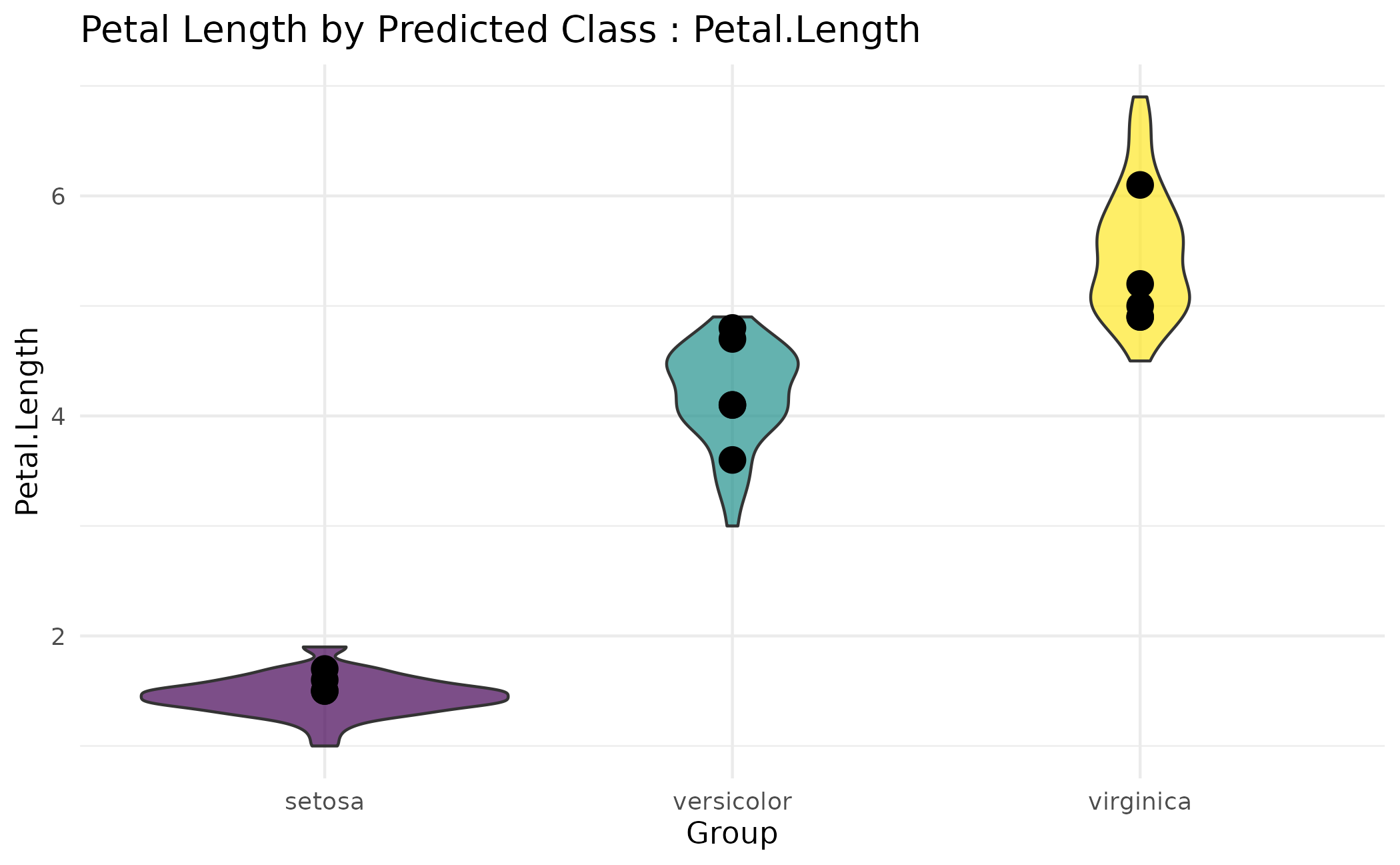

Combining Modules with honeycombHIVE

The R6 API with modules and the functional honeycombHIVE() API serve different use cases. For maximum control, use AINet directly with modules for single-pass analysis. For hierarchical refinement, use honeycombHIVE() with its built-in layer management and gradient refinement.

A typical advanced workflow:

Explore with bHIVE() to establish baseline performance
Tune with swarmbHIVE() to find good hyperparameters
Compose modules via AINet to add biological mechanisms
Layer with honeycombHIVE() for hierarchical refinement
Visualize with visualizeHIVE() to understand results

sessionInfo()

## R version 4.6.1 (2026-06-24)
## Platform: x86_64-pc-linux-gnu
## Running under: Ubuntu 24.04.4 LTS
## 
## Matrix products: default
## BLAS:   /usr/lib/x86_64-linux-gnu/openblas-pthread/libblas.so.3 
## LAPACK: /usr/lib/x86_64-linux-gnu/openblas-pthread/libopenblasp-r0.3.26.so;  LAPACK version 3.12.0
## 
## locale:
##  [1] LC_CTYPE=C.UTF-8       LC_NUMERIC=C           LC_TIME=C.UTF-8       
##  [4] LC_COLLATE=C.UTF-8     LC_MONETARY=C.UTF-8    LC_MESSAGES=C.UTF-8   
##  [7] LC_PAPER=C.UTF-8       LC_NAME=C              LC_ADDRESS=C          
## [10] LC_TELEPHONE=C         LC_MEASUREMENT=C.UTF-8 LC_IDENTIFICATION=C   
## 
## time zone: UTC
## tzcode source: system (glibc)
## 
## attached base packages:
## [1] stats     graphics  grDevices utils     datasets  methods   base     
## 
## other attached packages:
## [1] caret_7.0-1       lattice_0.22-9    viridis_0.6.5     viridisLite_0.4.3
## [5] ggplot2_4.0.3     bHIVE_0.99.6      BiocStyle_2.40.0 
## 
## loaded via a namespace (and not attached):
##  [1] pROC_1.19.0.1        gridExtra_2.3.1      rlang_1.2.0         
##  [4] magrittr_2.0.5       otel_0.2.0           e1071_1.7-17        
##  [7] compiler_4.6.1       png_0.1-9            systemfonts_1.3.2   
## [10] vctrs_0.7.3          reshape2_1.4.5       stringr_1.6.0       
## [13] pkgconfig_2.0.3      fastmap_1.2.0        labeling_0.4.3      
## [16] rmarkdown_2.31       prodlim_2026.03.11   ragg_1.5.2          
## [19] purrr_1.2.2          xfun_0.59            cachem_1.1.0        
## [22] jsonlite_2.0.0       recipes_1.3.3        BiocParallel_1.46.0 
## [25] clusterCrit_1.3.0    parallel_4.6.1       cluster_2.1.8.2     
## [28] R6_2.6.1             bslib_0.11.0         stringi_1.8.7       
## [31] RColorBrewer_1.1-3   reticulate_1.46.0    parallelly_1.47.0   
## [34] rpart_4.1.27         lubridate_1.9.5      jquerylib_0.1.4     
## [37] Rcpp_1.1.1-1.1       bookdown_0.47        iterators_1.0.14    
## [40] knitr_1.51           future.apply_1.20.2  Matrix_1.7-5        
## [43] splines_4.6.1        nnet_7.3-20          timechange_0.4.0    
## [46] tidyselect_1.2.1     yaml_2.3.12          timeDate_4052.112   
## [49] codetools_0.2-20     listenv_1.0.0        tibble_3.3.1        
## [52] plyr_1.8.9           withr_3.0.3          S7_0.2.2            
## [55] askpass_1.2.1        evaluate_1.0.5       Rtsne_0.17          
## [58] future_1.70.0        desc_1.4.3           survival_3.8-6      
## [61] proxy_0.4-29         pillar_1.11.1        BiocManager_1.30.27 
## [64] foreach_1.5.2        stats4_4.6.1         generics_0.1.4      
## [67] scales_1.4.0         globals_0.19.1       class_7.3-23        
## [70] glue_1.8.1           tools_4.6.1          data.table_1.18.4   
## [73] RSpectra_0.16-2      ModelMetrics_1.2.2.2 gower_1.0.2         
## [76] fs_2.1.0             grid_4.6.1           umap_0.2.10.0       
## [79] ipred_0.9-15         nlme_3.1-169         cli_3.6.6           
## [82] textshaping_1.0.5    lava_1.9.1           dplyr_1.2.1         
## [85] gtable_0.3.6         sass_0.4.10          digest_0.6.39       
## [88] htmlwidgets_1.6.4    farver_2.1.2         htmltools_0.5.9     
## [91] pkgdown_2.2.0        lifecycle_1.0.5      hardhat_1.4.3       
## [94] openssl_2.4.2        MASS_7.3-65

Nick Borcherding

2026-06-26